Tools Menu
11.12 Network Least Squares: SurvNET
FUNCTION: SurvNET performs a least squares adjustment and statistical analysis on a network of raw survey field data, including both total station measurements and GPS vectors. SurvNET simultaneously adjusts a network of interconnected traverses with any amount of redundancy. The raw data can contain any combination of traverse (angle and distance), triangulation (angle only) and trilateration (distance only) measurements, as well as GPS vectors. The raw data does not need to be in any specified order, and individual traverses do not have to be defined using any special codes. All measurements are used in the adjustment.
Activate SurvNET routine by picking from the Tools menu; or by pressing [Alt][T], [N]. SurvNET may also be activated from the Edit Process Raw File routines: under the Carlson Raw Editor (see Section 11.11) by pressing [Alt][T], [E], [A] then select Process > Least Squares; and under the C&G Raw Editor (see Section 11.10) by pressing [Alt][T], [E], [C] then select Tools > Network Least Squares.
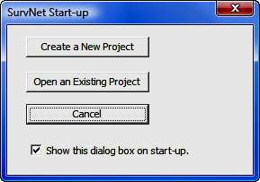
SurvNET is a project based program. Before performing a least squares adjustment an existing project must be opened or a new project needs to be created. The opening dialog box (shown above) allows the user to open or create a project on start-up. You also can create or open a project from the Files menu. Since all project management functions can be performed from the Files menu this start-up dialog box is a convenience and you may elect to turn it off by un-checking Show this dialog box on start-up.
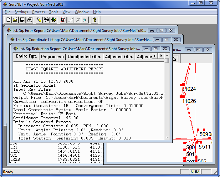
Shown below is the SurvNET main window with an existing project opened.
SurvNET reduces survey field measurements to grid coordinates in assumed, UTM, SPC83 SPC27, and a variety of other coordinate systems. In the 2D/1D model, a grid factor is computed for each individual line during the reduction. The elevation factor is computed for each individual line if there is sufficient elevation data. If the raw data has only 2D data, the user has the option of defining a project elevation to be used to compute the elevation factor.
SurvNET supports a variety of map projections and coordinate systems including the New Brunswick Survey Control coordinate system, UTM, and user defined systems consisting of either a predefined ellipsoid or a user defined ellipsoid and one of the following projections, Transverse Mercator, 1 Standard Parallel Lambert Conformal, 2 Standard Parallel Lambert Conformal, Oblique Mercator, and the Double Stereographic projection.
A full statistical report containing the results of the least squares adjustment is produced and written to the report file (.RPT). An error report file (.ERR) is created and contains any error messages that are generated during the adjustment.
Coordinates can be stored in a Carlson file (.CRD), C&G file (.CRD), Simplicity file (.ZAK) or an LDD file (.MDB). An ASCII coordinate file (.NEZ) is always created that can be imported into most any mapping/surveying/GIS program. The user has the option to compute unadjusted preliminary coordinates.
There is an option to compute traverse closures during the preprocessing of the raw data. Closures can be computed for both GPS loops and total station traverses. Closure for multiple traverse loops in the same raw file can be computed.
SurvNET can combine GPS vectors and total station data in a single adjustment. GPS Vector files from Leica, Thales, Topcon and Trimble can be input, as well as GPS files in the StarNet format. Additionally GPS vectors can be read from NGS G-files. There is also an option to read the G-file section of an Opus report.
SurvNET includes a variety of blunder detection routines. One blunder detection method is effective in detecting if the same point number has been used for two different points. Additionally this blunder detection method is effective in detecting if two different point numbers have been used for the same physical position. This method also flags other raw data problems. Another blunder detection method included in SurvNET is effective in isolating a single blunder, distance or angle in a network. This method does not require that there be a lot of redundancy, but is effective if there is only one blunder in the data set. Additionally, SurvNET includes a blunder detection method that can isolate multiple blunders, distances or angles in a network. This method does require that there be a lot of redundancy in the network to effectively isolate the multiple blunders.
Other key features include: Differential and Trig level networks and loops can be adjusted using the network least squares program. Geoid modeling is used in SurvNET, allowing the users to choose between the Geoid99 and the Geoid03 model. The user can alternately enter the project geoid separation. There are description codes to identify duplicate points with different point numbers. The user can specify the confidence interval from 50 to 99 percent.
SurvNET performs a least squares adjustment and statistical analysis of a network of raw survey field data, including both total station measurements, differential level data and GPS vectors. SurvNET simultaneously adjusts a network of interconnected traverses with any amount of redundancy. The raw data can contain any combination of angle and distance measurements, and GPS vectors. SurvNET can adjust any combination of trilaterations, traverses, triangulations, networks and resections. The raw data does not need to be in a linear format, and individual traverses do not have to be defined using any special codes. All measurements are used in the adjustment.
Least squares is very flexible in terms of how the survey data needs to be collected. Generally speaking, any combination of angles, and distances combined with a minimal amount of control points and azimuths are needed. This data can be collected in any order. There needs to be at least some redundancy in the measurements. Redundant measurements are measurements that are in excess of the minimum number of measurements needed to determine the unknown coordinates. Redundancy can be created by including multiple GPS and other control points within a network or traverse. Measuring angles and distances to points in the network that have been located from another point in the survey creates redundancy. Running additional cut-off traverses or additional traverses to existing control points creates redundancy. Following are some general rules and tips in collecting data for least squares reduction.
Backsights should be to point numbers. Some data collectors allow the user to backsight an azimuth not associated with a point number. SurvNET requires that all backsights be associated with a point number.
There has to be at least a minimum amount of control. There has to be at least one control point. Additionally there needs to be either one additional control point or a reference azimuth. Control points can be entered in either the raw data file or there can be a supplemental control point file containing the control point. Reference azimuths are entered in the raw data file. The control points and reference azimuths do not need to be for the first points in the raw file. The control points and azimuths can be associated with any point in the network or traverse. The control does not need to be adjacent to each other. It is permissible, though unusual, to have one control point on one side of the project and a reference azimuth on the other side of the project.
Some data collectors do not allow the surveyor to shoot the same point twice using the same point number. SurvNET requires that all measurements to the same point use a single point number. The raw data may need to be edited after it has been downloaded to the office computer to insure that points are numbered correctly. An alternative to renumbering the points in the raw data file is to use the 'Pt Number substitution string' feature in the project 'Settings' screen. See the 'Redundant Measurement' section for more details on this feature.
The majority of all problems in processing raw data are related to point numbering problems. Using the same point number twice to different points, not using the same point number when shooting the same point, misnumbering backsights or foresights, and misnumbering control points are all common problems.
A big source of problems with new users is a misunderstanding in defining their control for a project. It is always best to explicitly define the control for the project. A good method is to put all the control for a project into a separate raw file.
Some raw data collector files may have preliminary unadjusted coordinates included with the raw data. These coordinate records should be removed from the raw file. The only coordinate values that should be in the raw file are the control points. Since there is no concept of 'starting coordinates' in least squares there is no way for SurvNET to determine which points are considered control and which points are preliminary unadjusted points. So all coordinates found in a raw data file will be considered control points.
When a large project is not processing correctly, it is often useful to divide the project into several raw data files and debug and process each file separately as it is easier to debug small projects. Once the smaller projects are processing separately they can be combined for a final combined adjustment.
SurvNET gives the user the option to choose one of two mathematical model options when adjusting raw data, the 3D model and the 2D/1D model.
In the process of developing SurvNET, numerous projects have be adjusted using both the 2D/1D model and the 3D model. There are slight differences in final adjusted coordinates when comparing the results from the same network using the two models. But in all cases the differences in the results are typically less than the accuracy of measurements used in the project. The main difference in terms of collecting raw data for the two different models is that the 3D model requires that rod heights and instrument heights need to be measured, and there needs to be sufficient elevation control to compute elevations for all points in the survey. When collecting data for the 2D/1D model the field crews do not need to collect rod heights and instrument heights.
In the 2D/1D model raw distance measurements are first reduced to horizontal distances and then optionally to grid distances. Then a two dimensional horizontal least squares adjustment is performed on these reduced horizontal distance measurements and horizontal angles. After the horizontal adjustment is performed an optional one-dimensional vertical least squares adjustment is performed in order to adjust the elevations if there is sufficient data to compute elevations. The 2D/1D model is the model that has been traditionally been used in the past by non-geodetic surveyors in the reduction of field data. There are several advantages of SurvNET's implementation of the 2D/1D model. One advantage is that an assumed coordinate system can be used. It is not necessary to know geodetic positions for control points. Another advantage is that 3D raw data is not required. It is not necessary to record rod heights and heights of instruments. Elevations are not required for the control points. The primary disadvantage of SurvNET's implementation of the 2D/1D model is that GPS vector data cannot be used in 2D/1D projects.
In the 3D model raw data is not reduced to a horizontal plane prior to the least squares adjustment. The 3 dimensional data is adjusted in a single least squares process. In SurvNET's implementation of the 3D model XYZ geodetic positions are required for control. The raw data must contain full 3D data including rod heights and measured heights of instrument. The user must designate a supported geodetic coordinate system. The main advantage of using the 3D model is that GPS vectors can be incorporated into the adjustment. Another advantage of the 3D model is the ability to compute and adjust 3D points that only have horizontal and vertical angles measured to the point. This feature can be used in the collection of points where a prism cannot be used, such as a power line survey.
When using the 2D/1D model if you have Vertical Adjustment turned ON in the project settings, elevations will be calculated and adjusted only if there is enough information in the raw data file to do so. Least squares adjustment is used for elevation adjustment as well as the horizontal adjustment. To compute an elevation for the point the instrument record must have a HI, and the foresight record must have a rod height, slope distance and vertical angle. If working with .CGR raw data a 0.0 (zero) HI or rod height is valid. It is only when the field is blank that the record will be considered a 2D measurement. Carlson SurvCE 2.0 or higher allows you to mix 2D and 3D data by inserting a 2D or 3D comment record into the .RW5 file. A 3D traverse must also have adequate elevation control in order to process the elevations. Elevation control can be obtained from the supplemental control file, coordinate records in the raw data file, or elevation records in the raw data file.
SurvNET can also automatically reduce field measurements to state plane coordinates in either the NAD 83 or NAD 27 or other supported geodetic coordinate systems. In the 2D/1D model a grid factor is computed for each individual line during the reduction. The elevation factor is computed for each individual line if there is sufficient elevation data. If the raw data has only 2D data, the user has the option of defining a project elevation to be used to compute the elevation factor.
A full statistical report containing the results of the least squares adjustment is produced and written to the report file (.RPT). An error report file (.ERR) is created and contains any error messages that are generated during the adjustment. Coordinates can be stored in the following formats:
C&G numeric (*.crd)
C&G alphanumeric (*.cgc)
Carlson numeric (*.crd)
Carlson alphanumeric (*.crd)
Autodesk Land Desktop (*.mdb)
Simplicity (*.zak)
ASCII P,N,E,Z,D,C (*.nez)
A file with the extension .OUT is always created and contains an ASCII formatted coordinate list of the final adjusted coordinates formatted suitable for printing. Additionally an ASCII file with an extension of .NEZ containing the final adjusted coordinates in a format suitable for input into 3rd party software that is capable of inputting an ASCII coordinate file.
SurvNET produces a wealth of statistical information that allows an effective way to evaluate the quality of survey measurements. In addition to the least squares statistical information there is an option to compute traverse closures during the preprocessing of the raw data. Traverse closures can be computed for both GPS loops and total station traverses. This option has no effect on the computation of final least squares adjusted coordinates. This option is useful for surveyors who due to statutory requirements are still required to compute traverse closures and for those surveyors who still like to view traverse closures prior to the least squares adjustment.
SurvNET works equally well for raw file formats from both Carlson and C&G. The primary difference between the two is that a Carlson user will typically be using an .RW5 file for his raw data and a C&G user will typically be using a .CGR as the source of his raw data.
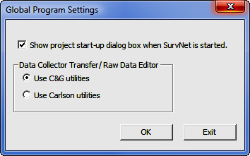
SurvNET is capable of processing either C&G raw data files (.CGR) or Carlson raw data files (.RW5). Measurement, coordinate, elevation and direction (Brg/Az) records are all recognized. Scale factor records in the .CGR file are not processed since SurvNET calculates the state plane scale factors automatically. The menu option Global Settings displays the following dialog box. If Use Carlson Utilities is chosen then the Carlson Editor (.RW5) will be the default raw editor and Carlson SurvCom will be the default data collection transfer program. If Use C&G Utilities is chosen then the C&G Editor (.CGR) will be the default raw editor and C&G's Transfer program will be the default data collection transfer program.
Standard errors are estimated errors that are assigned to measurements or coordinates. A standard error is an estimate of the standard deviation of a sample. A higher standard error indicates a less accurate measurement. The higher the standard error of a measurement, the less weight it will have in the adjustment process.
Although you can set default standard errors for the various types of measurements in the project settings of SurvNET, standard errors can also be placed directly into the raw data file. A standard error record inserted into a raw data file controls all the measurements following the SE record. The standard error does not change until another SE record is inserted that either changes the specific standard error, or sets the standard errors back to the project defaults. The advantage of entering standard errors into the raw file is that you can have different standard errors for the same type measurement in the same job. For example, if you used a one second total station with fixed backsights and foresights for a portion of a traverse and a 10 second total station with backsights and foresights to hand held prisms on the other portion of the traverse, you would want to assign different standard errors to reflect the different methods used to collect the data.
Make sure the SE record is placed before the measurements for which it applies.
If you do not have standard errors defined in the raw data file, the default standard errors in the project settings will be applied to the entire file.
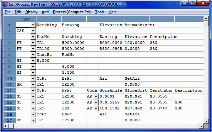
The raw data editor can be accessed from the tool bar icon. Following is an image of the .RW5 editor. Refer to the Carlson raw editor documentation for guidance in the basic operation of the editor. The following documentation only deals with topics that are specific to the .RW5 editor and SurvNET.
You can insert or add standard error records into the raw data file. Use the INSERT or ADD menu option and select Standard Errors, or pick the SE buttons on the tool bar. Use the Add menu option to insert standard error records into the raw files.
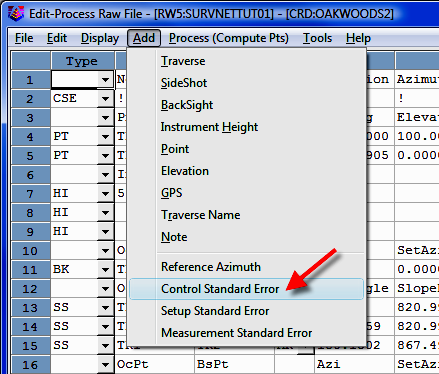
You can set standard errors for Northing, Easting, Elevation, and Azimuth using the Control Standard Error menu option. Azimuth standard errors are entered in seconds. The North, East and Elevation standard errors affect the PT (coordinate) and EL (elevation) records.
You can hold or FIX the North, East and Elevation fixed by entering a "!" symbol. You can allow the North, East and Elevation to FLOAT by entering a "#" symbol. You can also assign the North, East and Elevation actual values. If you use an "*" symbol, the current standard error values will revert to the project default values.
North East
Elevation Azim
! ! !
(Fix all values)
# # # 30.0 (Allow
the N., E. & Elevation to Float)
0.01 0.01 0.03 5.0
(assign values)
* * * *
(return the standard errors back to
project defaults)
When you fix a measurement, the original value does not change during the adjustment and all other measurements will be adjusted to fit the fixed measurements. If you allow a value to float, it will not be used in the actual adjustment, it will just be used to help calculate the initial coordinate values required for the adjustment process. Placing a very high or low standard error on a measurement accomplishes almost the same thing as setting a standard error as fixed or float. The primary purpose of using a float point is if SurvNET cannot compute preliminary values, a preliminary float value can be computed and entered for the point.
Direction records cannot be FIXED or FLOAT. You can assign a low standard error (or zero to fix) if you want to weight it heavily, or a high standard error to allow it to float.
Example:
North East Elev Azim
CSE
! ! !
PT 103 1123233.23491 238477.28654 923.456
PT 204 1124789.84638 239234.56946 859.275
PT 306 1122934.25974 237258.65248 904.957
North East Elev Azim
CSE * * *
PT 478 1122784.26874 237300.75248 945.840
The first SEc record containing the "!" character and sets points 103, 204, and 306 to be fixed. The last SEc record contains the "*" character. It sets the standard errors for point 478 and any other points that follow to the project settings. The Azimuth standard error was left blank.
You can set the standard errors for distances, horizontal angle pointing, horizontal angle reading, vertical angle pointing, vertical angle reading, and distance constant and PPM.
Distance - distance constant and measurement error, can be obtained from EDM specs, or from performing an EDM calibration on an EDM baseline, or from other testing done by the user.
PPM - Parts per Million, obtain from EDM specs, or from performing an EDM calibration on an EDM baseline, or from other testing done by the user.
Pointing - total station horizontal angular pointing error in seconds. This value is an indication of how accurately the instrument man can point to the target. For example, you may set it higher in the summer because of the heat waves; or you may set it higher for total stations running in Robotic Mode because they cannot point as well as a manual sighted total station.
Reading - total station horizontal angular reading error in seconds. If you have a 10 second theodolite, enter a reading error of 10 seconds.
V.Pointing - total station vertical angular pointing error in seconds. This value is an indication of how accurately the instrument man can point to the target. For example, you may set it higher in the summer because of the heat waves.
V.Reading - total station vertical angular reading error in seconds. If you have a 10 second theodolite, enter a reading error of 10 seconds.
Example:
Distance Point Read V.Point V.Read PPM
MSE 0.01 3 3 3 3 5
You can enter any combination of the above values. If you do not want to change the standard error for a particular measurement type, leave it blank.
If you use an "*" symbol, the standard error for that measurement type will return to the project default values.
These standard errors are a measure of how accurately the instrument and target can be setup over the points.
Rod Ctr is the Target Centering error. This value reflects how accurately the target prism can be set up over the point.
Inst Ctr is the Instrument Centering error. This value reflects how accurately the instrument can be set up over the point.
Ints Hgt is the Instrument Height error. This value reflects how accurately the height of the instrument above the mark can be measured.
Rod Hgt is the Target Height error. This value reflects how accurately the height of the prism above the mark can be measured.
Example:
TargCtr InstCtr HI TargHgt
SSE 0.005 0.005 0.01 0.01
You can enter any combination of the above values. If you do not want to change the standard error for a particular measurement type, leave it blank.
If you use an "*" symbol, it will return the standard error to the project default values.
You can set standard errors for control, measurements and instrument setup using the Insert > Standard Error menu option:
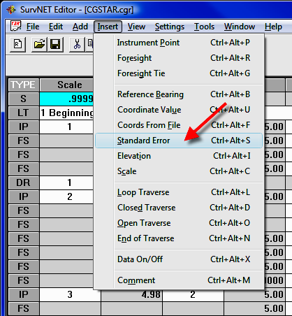
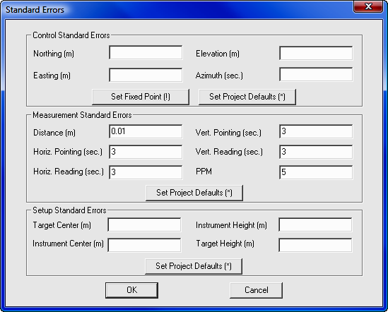
This will open a Standard Errors dialog box:
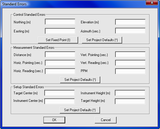
This dialog allows you to create three types of standard error records: Control, Measurement, and Setup. You need only enter the values for the standard errors you wish to set. If a field is left blank no standard error for that value will be inserted into the raw data file.
You can FIX the North, East and Elevation by entering a "!" symbol (as shown above). You can allow the North, East and Elevation to FLOAT by entering a "#" symbol. You can also assign the North, East and Elevation actual values. (In the 2D/1D model elevation control is ALWAYS fixed.) If you use an "*" symbol (or press the [Set Project Defaults] button), the current standard error value will return to the project default values.
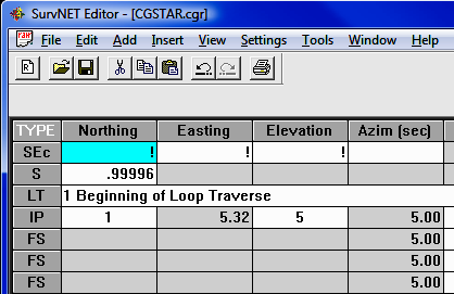
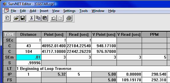
In the above example, a Control Standard Error record (SEc) will be created:
Below are some sample values for control standard errors:
North East
Elevation Azim
! ! ! (Fix
all values)
# # #
30.0 (Allow the N., E. & Elevation
to Float)
0.01 0.01 0.03 5.0
(assign values)
* * *
* (return the standard errors
back to project defaults)
When you fix a measurement, the original value does not change during the adjustment and all other measurements will be adjusted to fit the fixed measurements. If you allow a value to float, it will not be used in the actual adjustment, it will just be used to help calculate the initial coordinate values required for the adjustment process. Placing a very high or low standard error on a measurement accomplishes almost the same thing as setting a standard error as float or fixed. The primary purpose of using a float point is if SurvNET cannot compute preliminary values, a preliminary float value can be computed and entered for the point.
Direction records cannot be FIXED or FLOAT. You can assign a low standard error (or zero to fix) if you want to weight it heavily, or a high standard error to allow it to float.
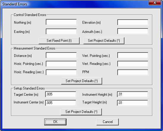
You can set the standard errors for distances, horizontal angle pointing, horizontal angle reading, vertical angle pointing, vertical angle reading, and distance constant and PPM.
Distance - distance constant and measurement error, can be obtained from EDM specs, or from performing an EDM calibration on an EDM baseline, or from other testing done by the user.
PPM - Parts per Million, obtain from EDM specs, or from performing an EDM calibration on an EDM baseline, or from other testing done by the user.
Pointing - total station horizontal angular pointing error in seconds. This value is an indication of how accurately the instrument man can point to the target. For example, you may set it higher in the summer because of the heat waves; or you may set it higher for total stations running in Robotic Mode because they cannot point as well as a manual sighted total station.
Reading - total station horizontal angular reading error in seconds. If you have a 10 second theodolite, enter a reading error of 10 seconds.
V. Pointing - total station vertical angular pointing error in seconds. This value is an indication of how accurately the instrument man can point to the target. For example, you may set it higher in the summer because of the heat waves.
V. Reading - total station vertical angular reading error in seconds. If you have a 10 second theodolite, enter a reading error of 10 seconds.
Example:
You can enter any combination of the above values. If you do not want to change the standard error for a particular measurement type, leave it blank. If you use an "*" symbol, the standard error for that measurement type will return to the project default values.
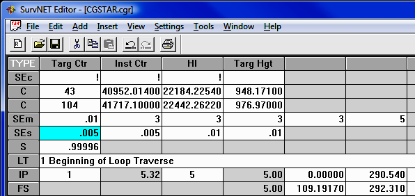
The following SEm record will be created:
These standard errors are a measure of how accurately the instrument and target can be setup over the points.
Targ Ctr is the Target Centering error. This value reflects how accurately the target prism can be set up over the point.
Inst Ctr is the Instrument Centering error. This value reflects how accurately the instrument can be set up over the point.
HI is the Instrument Height error. This value reflects how accurately the height of the instrument above the mark can be measured.
Targ Hgt is the Target Height error. This value reflects how accurately the height of the prism above the mark can be measured.
Example:
You can enter any combination of the above values. If you do not want to change the standard error for a particular measurement type, leave it blank.
If you use an "*" symbol, it will return the standard error to the
project default values.
The following SEs record will be created:
There are several other features available in both the Carlson and C&G editors that are useful to SurvNET.
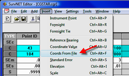
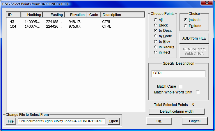
Insert Coordinate records from file - when inputting control into a raw data file, it is more convenient to read the control point directly from a coordinate file than it is to manually key them in. The Insert Coordinates function allows you to select points in a variety of manner making it easy to select just control points. For example, you can select points by description, code, point blocks, point number, etc.
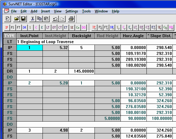
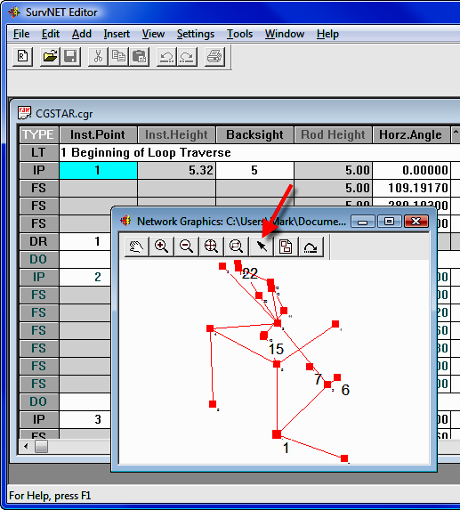
Data ON/OFF records - when trying track down problems, sometimes it is convenient to remove certain sections of raw data prior to processing. The editors have a special record (DO record) that will turn OFF or ON certain areas of data. For example, when you insert a DO record all data following that record will be turned OFF (it will be shown in a different color). When you insert another DO record further down, the data following it will be turn back ON. It is simply a toggle. In the example below, the instrument setup at point 2 back sighting 1 was turned OFF.
Graphics and the C&G Editor - When using the C&G editor the graphics window can be used to navigate within the raw data. To use this feature initiate the graphics window from the C&G Editor.
Click the graphic Pick Point button then pick the desired point in the graphic window. The text editor cursor should move to the next record that contains that point number.
If there is more than one point number within the search radius a dialog box is displayed so that the desired point can be chosen.
One of the benefits of least squares is the ability to process redundant measurements. In terms of total station data, redundant measurement is defined as measuring angles and/or distances to the same point from two or more different setups.
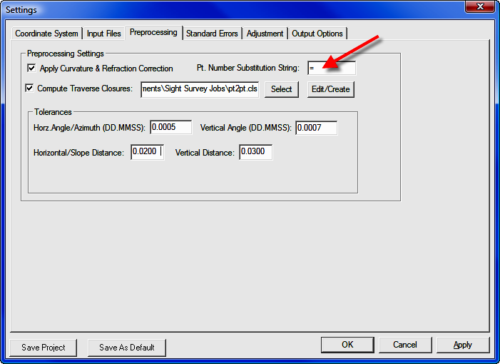
It is required that the same point number be used when locating a point that was previously recorded. However, since some data collectors will not allow you to use the same point number if the point already exists, the following convention for collecting redundant points while collecting the data in the field is used. If you begin the point description with a user defined string, for example a "=" (equal sign) followed by the original point number, that measurement will be treated as a redundant measurement to the point defined in the description field. The user defined character or string is set in the project settings dialog. For example, if point number 56 has the description "=12", we will treat point number 56 as a shot to point number 12, not point 56. Make sure the Settings > Project Settings > Preprocessing Settings dialog box has the Pt. Number Substitution String set to the appropriate value.
Alternately, the point numbers can be edited after the raw data has been downloaded from the data collector.
Select Settings > Project Settings > Input Files to set Supplemental Control Files.
In order to process a raw data file, you must have as a minimum a control point and a control azimuth, or two control points. Control points can be inserted into the raw data file or alternately control points can be read from coordinate files. Control points can be read from a variety of coordinate file types:
C&G or Carlson numeric (.CRD) files
C&G Alphanumeric coordinate files (*.cgc)
Carlson Alphanumeric coordinate files (*.crd)
Autodesk Land Desktop (*.mdb)
Simplicity coordinate files (*.zak)
ASCII (.NEZ) file
ASCII latitude and longitude (3D model only)
CSV ASCII NEZ with std. errors
Typically the standard errors for the control points from a supplemental control file will be assigned from the NORTH, and EAST standard errors from the project settings dialog box. The option CSV ASCII NEZ with std. is the exception. With this option the standard errors are field within the file.
In the ASCII .NEZ file, the coordinate records need to be in the following format:
Pt. No., Northing,
Easting, Elevation, Description<cr><lf>
103, 123233.23491, 238477.28654, 923.456, Mon 56-7B<CR><LF>
Each line is terminated with carriage-return <CR> and line-feed <LF> characters.
In the ASCII latitude and longitude file, the records need to be in the following format:
Pt.No., Lat.(NDDD.mmssssss),
Lon.(WDDD.mmssssss),Elev.(Orthometric), Desc.<cr><lf>
FRKN, N35.113068642, W083.234174724, 649.27<CR><LF>
Each line is terminated with carriage-return <CR> and line-feed <LF> characters.
In the CVS ASCII .NEZ with std. errors file, the coordinate records need to be in the following format: This format is typically created as an output NEZ option. The typical use of this format is if the control for a project was initially created as a project. Then the points from that projects can be used as supplemental control for subsequent projects and the actual standard errors of the control will be used.
Pt.No., Northing,
Easting, Elevation, Std.Err.N, Std.Err.E, Std.Err.Z, Description<cr><lf>
504, 204015.23528803, 786760.95695104, 876.15662064, 0.002, 0.003, 0.004, ,
1<CR><LF>
Each line is terminated with carriage-return <CR> and line-feed <LF> characters.
The major advantage of putting coordinate control points in the actual raw data file is that specific standard errors can be assigned to each control point (as described in the RAW DATA section above). If you do not include an SE record the standard error will be assigned from the NORTH, EAST, and ELEVATION standard errors from the project settings dialog box.
|
|
WARNING: The supplemental control file and the final output file should never be the same. Since least squares considers all points to be control points only control points should be in a supplemental control file. If the supplemental control file has coordinate values for points that are not control points then these coordinate values will still be treated as control. |
Most least squares operations are initiated from the main network least squares window.
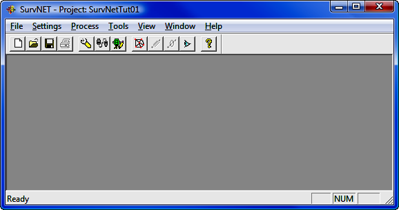
Selecting the FILE menu option opens the following menu:
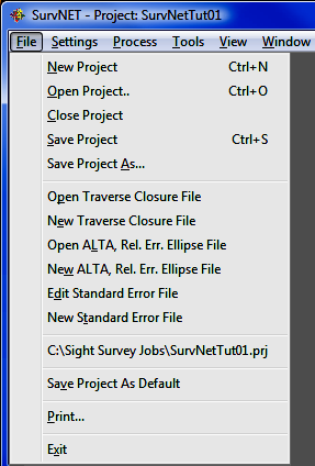
A Project File (.PRJ) is created in order to store all the settings and files necessary to reprocess the data making up the project. You can create a NEW project, or OPEN an existing project. It is necessary to have a project open in order to process the data.
Save Project As Default can be used to create default project settings to be used when creating a new project. The current project settings are saved and will be used as the default settings when any new project is created.
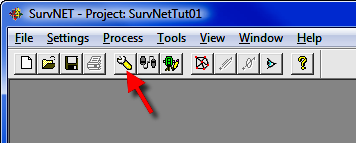
The project settings are set by selecting Settings > Project Settings from the menu, or pressing the SE icon on the tool bar.
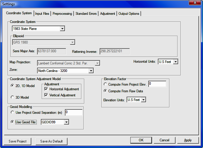
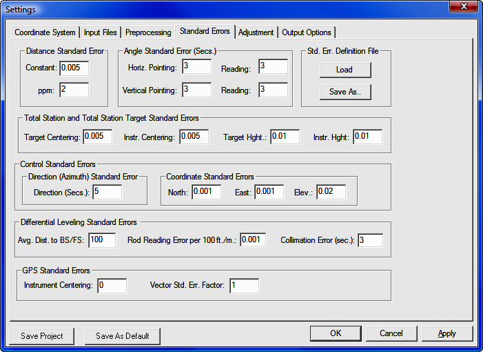
The project settings dialog box has six tabbed windows, Coordinate System, Input Files, Preprocessing, Adjustment, Standard Errors, and Output Options.
Notice that there are two buttons at the lower left of the dialog box. The [Save Project] button can be used to store the current settings to the active project. If there is no active project then the user will be prompted for a new project file name. Projects can also be saved using the File > Save Project menu option from the main menu. The [Save as Default] button can be used to save the current project settings as the default settings whenever a new project is created. Default project settings can also be defined using the File > Save Project as default menu option from the main menu.
The Coordinate System tab contains settings that relate to the project coordinate system, output units, the adjustment model and other geodetic settings.
You can select either the 3D model or the 2D/1D mathematical model. If you choose 2D/1D mathematical model you can choose to only perform a horizontal adjustment, a vertical adjustment or both. In the 3D model both horizontal and vertical are adjusted simultaneously. The 3D model requires that you choose a geodetic coordinate system. Local, assumed coordinate systems cannot be used with the 3D model. GPS vectors can only be used when using the 3D model.
If using the 2D/1D mathematical model you can select Local (assumed coordinate system), or a geodetic coordinate system such State Plane NAD83, State Plane NAD27, UTM, or a user-defined coordinate system as the coordinate system. When using the 3D model you cannot use a local system.
Select the Horizontal Units for output of coordinate values (Meters, US Feet, or International Feet). In the 3D model both horizontal and vertical units are assumed to be the same. In the 2D/1D model horizontal and vertical units can differ. The Horizontal Units setting in this screen refers to the output units. It is permissible to have input units in feet and output units in meters. Input units are set in the Input Files tabbed screen.
If you choose SPC 1983, SPC 1927, or UTM, the appropriate zone will need to be chosen. The grid scale factor is computed for each measured line using the method described in Section 4.2 of NPAA Manual NOS NGS 5, "State Plane Coordinate System of 1983", by James E. Stem.
If using the 2D/1D model and you select a geodetic coordinate system, you have a choice as to how the elevation factor is computed. You can choose to either enter a project elevation or you can choose to have elevations factors computed for each distance based on computed elevations. In order to use the Elevation Factor: Compute from Raw Data all HI's and foresight rod heights must be collected for all points.
If you choose a geodetic coordinate system and are using the 2D/1D model you will want to select Compute from Project Elevation if any of your raw data measurements are missing any rod heights or instrument heights. There must be enough information to compute elevations for all points in order to compute elevation factors. For most survey projects it is sufficient to use an approximate elevation, such as can be obtained from a Quad Sheet for the project elevation.
If you are using either the 3D or the 2D/1D adjustment model using SPC 1983 or UTM reduction you must choose a geoid modeling method. A project geoid separation can be entered or the GEOID99 or GEOID03 grid models can be used. The project must fall within the geographic range of the geoid grid files in order to use GEOID99 or GEOID03 models.
Geoid modeling is used as follows. Entering a 0.0 value for the separation is the method to use if you wish to ignore the geoid separation. In the 2D, 1D model it is assumed that elevations entered as control are entered as orthometric heights. Since grid reduction requires the data be reduced to the ellipsoid, the geoid separation is used to compute ellipsoid elevations. The difference between using geoid modeling and not using geoid modeling or using a project geoid separation is insignificant for most surveys of limited extents. In the 3D model it is also assumed that elevations entered as control are orthometric heights. Since the adjustment is performed on the ellipsoid, the geoid separation is used to compute ellipsoid elevations prior to adjustment. After the adjustment is completed the adjusted orthometric elevations will be computed from the adjusted ellipsoid elevations and the computed geoid separation for each point.
Geoid modeling is especially important for projects covering large extents. If you incorporate GPS vector data from an OPUS solution into your project it will be necessary to use geoid modeling, otherwise your results will be poor.
If you choose the GEOID99 or GEOID03 modeling option, geoid separations are computed by interpolation with data points retrieved from geoid separation files. The geoid separation files should be found in the primary the installation directory. Grid files have an extension of .GRD. These files should have been installed during the installation of SurvNET. These files can be downloaded from the Carlson/C&G website, www.carlsonsw.com, if needed. The geoid files used by SurvNET are not in the same format as the geoid files available from NGS. The geoid files used by SurvNET must come from Carlson/C&G, either installed during installation or downloaded from the Carlson website.
If you choose to enter a project geoid separation the best way to determine a project geoid separation is by using the GEOID03 option of the NGS on-line Geodetic Toolkit. Enter a latitude and longitude of the project midpoint and the program will output a project separation.
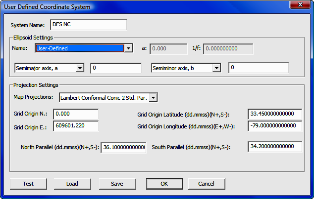
SurvNET allows the creation of user-defined geodetic coordinate systems (UDP). The ability to create user-defined coordinate system allows the user to create geodetic coordinate systems based on projections that are not explicitly supported by SurvNET. A SurvNET user-defined coordinate system consists of an ellipsoid, and a map projection. The ellipsoid can be one of the explicitly supported ellipsoids or a user-defined ellipsoid. The supported map projections are Transverse Mercator, Lambert Conformal Conic with 1 standard parallel, Lambert Conformal Conic with 2 standard parallels, Oblique Mercator (NGS), and Double Stereographic projection. User-defined coordinate systems are created, edited, and attached to a project from the Project Settings: Coordinate System dialog box. To attach an existing UDP file (.UDP) to a project use the [Select] button. To edit an existing .UDP file or create a new .UDP file use the [Edit] button.
The User-defined Oblique Mercator projection used by SurvNET uses the Oblique Mercator projection formulas published in the NGS document "State Plane Coordinate System of 1983' by James Stem. This implementation of the Oblique Mercator projection uses the convention of the False North and East being the natural origin, as opposed to the origin being the center of the projection.
The following dialog box is used to create the user-defined coordinate system. The ellipsoid needs to be defined and the appropriate map projection and projection parameters need to be entered. The appropriate parameter fields will be displayed depending on the projection type chosen.
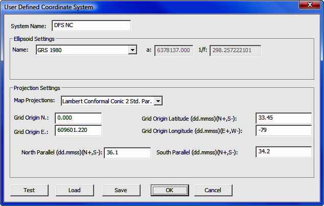
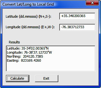
Test - Use the [Test] button to enter a known latitude and longitude position to check that the UDP is computing correct grid coordinates. Following is the test UDP dialog box. Enter the known lat/long in the top portion of the dialog box then press [Calculate] and the computed grid coordinates will be displayed in the Results list box.
Load -Use the [Load] to load the coordinate system parameters from an existing UDP.
Save - Use the [Save] button to save the displayed UDP. The [Save] button prompts the user to enter the UDP file name.
OK - Use the [OK] button to save the UDP using the existing file name and return to the Coordinate System dialog box.
Cancel - Use the [Cancel] button to return to the Coordinate System dialog box without saving any changes to the UDP file.
Ellipsoid Settings: User-Defined Ellipsoid - If you need to define an ellipsoid chose the User-Defined ellipsoid option. With the user-defined ellipsoid you will then have the option to enter two of the ellipsoid parameter.
Raw Data Files: Use the [Add] button to insert raw total station files into the list. Use the [Remove] button to remove raw files from the list. All the files in this list are included in the least squares adjustments. Having the ability to choose multiple files allows you to keep control in one file and measurements in another file, or different files collected at different times can be processed all at one time. If you have multiple crews working on the same project using different equipment, you can have "crew-specific" raw data files with standard error settings for their particular equipment. Having separate data files is also a convenient method of working with large projects. It is often easier to debug and process individual raw files. Once the individual files are processing correctly all the files can be included for a final adjustment. You can either enter C&G raw files (.CGR) or Carlson files (.RW5) into the list for processing. You cannot have both .CGR and .RW5 files in the same project to be processed at the same time. Notice that you have the ability to highlight multiple files when removing or adding files.
Level Raw Files: Differential and Trig level files can be entered and processed. Differential level raw files have an .LVL extension and are created using the Carlson/C&G level editor. Carlson SurvCE 2.0 or higher allows you to store differential or trig levels in a .TLV file which can also be processed by SurvNET.
GPS Vector Files: GPS vector files can be entered and processed. Both GPS vector files and total station raw files can be combined and processed together. You must have chosen the 3D Mathematical Model in the Coordinate System tab in order to include GPS vectors in the adjustment.
Currently, the following GPS vector file formats are supported.
Thales: Thales files typically have .obn extensions and are binary files.
Leica: Leica files are ASCII files.
StarNet ASCII GPS: See below for more information on StarNet format. These files typically have .GPS extensions.
Topcon (.tvf): Topcon .tvf files are ASCII files.
Topcon (.xml): Topcon also can output their GPS vectors in XML format which is in ASCII format.
Trimble Data Exchange Format (.asc): These files are in ASCII format.
Trimble data collection (.dc): These files are ASCII.
LandXML, (*.xml)
NGS G-File
NGS G-File from an OPUS report.
The following is a typical vector record in the StarNet ASCII format. GPS vectors typically consist of the "from" and "to" point number, the delta X, delta Y, delta Z values from the "from" and "to" point, with the XYZ deltas being in the geocentric coordinate system. Additionally the variance/covariance values of the delta XYZ's are included in the vector file.
G0 'V3 00:34 00130015.SSF
G1 400-401 4725.684625 -1175.976652 1127.564218
G2 1.02174748583350E-007 2.19210810829205E-007 1.23924502584092E-007
G3 6.06552466633441E-008 -5.58807795027874E-008 -9.11050726758263E-008
The G0 record is a comment. The G1 record includes the "from" and "to" point and the delta X, delta Y, and delta Z in the geocentric coordinate system. The G2 record is the variance of X,Y, and Z. The G3 record contains the covariance of XY, the covariance ZX, and the covariance ZY. Most all GPS vector files contain the same data fields in varying formats.
Use the [Add] button to insert GPS vector files into the list. Use the [Delete] button to remove GPS vector files from the list. All the files in this list will be used in the least squares adjustments. All the GPS files in the list must be in the same format. If the GPS file format is ASCII you have the option to edit the GPS vector files. The Edit option allows the editing of any of the ASCII GPS files using Notepad. Typically, only point numbers would be the fields in a GPS vector file that a user would have need to edit. The variance/covariance values are used to determine the weights that the GPS vectors will receive during the adjustment and are not typically edited.
For a variety of reasons it is common for GPS vector data collected with GPS equipment to have point names that do not match the point names used in the total station data. Generally the easiest way to handle this situation is to first convert the GPS data into the StarNet ASCII format using the Tools/Convert GPS file to ASCII menu option. Once the file has been converted to ASCII it is straightforward to change the G1 records using any text editor to reflect the correct point numbers.
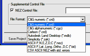
Supplemental Control File: The supplemental control file option allows the user to designate an additional coordinate file to be used as control. The supplemental control files can be from a variety of different file types.
C&G numeric (*.crd)
C&G alphanumeric (*.cgc)
Carlson numeric(*.crd)
Carlson alphanumeric(*.crd)
Autodesk Land Desktop (*.mdb)
Simplicity (*.zak)
ASCII P,N,E,Z,D,C (*.nez)
ASCII P,Lat,Long,Ortho,D,C (*.txt)
CSV ASCII NEZ with std. errors
Note: You should never use the same file for supplemental control points and for final output. Least squares considers all points to be measurements. If the output file is also used as a supplemental control file then after the project has been processed, all the points in the project would now be in the control file and all the points in the file would now be considered control points if the project was processed again. The simplest and most straight-forward method to define control for a project is to include the control coordinates in a raw data file.
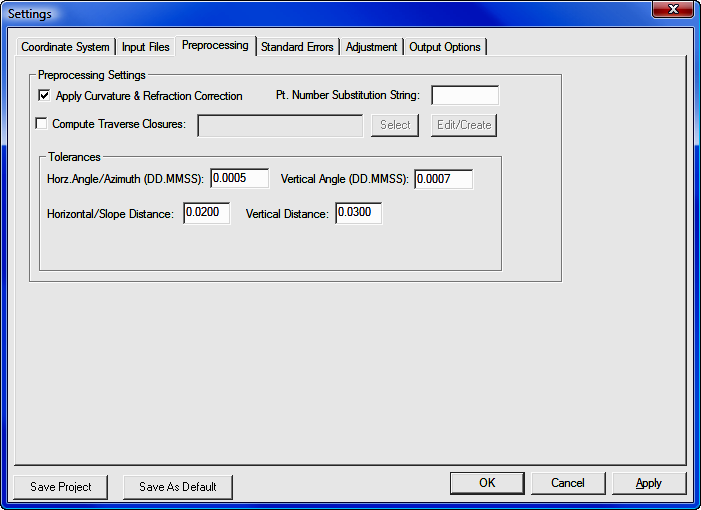
The Preprocessing tab contains settings that are used in the preprocessing of the raw data.
Apply Curvature and Refraction Corrections:
Set this toggle if you wish to have the curvature refraction correction
applied in the 2D/1D model when reducing the slope distance/vertical angle to
horizontal distance and vertical distance. Curvature and refraction
primarily impacts vertical distances.
Tolerances: When sets of angles
and/or distances are measured to a point, a single averaged value is calculated
for use in the least squares adjustment. You may set the tolerances so
that a warning is generated if any differences between the angle sets or
distances exceed these tolerances. Tolerance warnings will be shown in the
report (.RPT) and the (.ERR) file after processing the data.
Horz./Slope Dist Tolerance: This
value sets the tolerance threshold for the display of warnings if the difference
between highest and lowest horizontal distance exceeds this value. In the
2D model it is the horizontal distances that are being compared. In the 3D
model it is the slope distances that are being compared.
Vert. Dist Tolerance: This value sets the tolerance threshold for the display of a warning if the difference between highest and lowest vertical difference component exceeds this value (used in 2D model only).
Horz. Angle
Tolerance: This value sets the tolerance threshold for the display of
a warning if the difference between the highest and lowest horizontal angle
exceeds this value.
Vert. Angle Tolerance: This value sets the tolerance threshold for the
display a warning if the difference between the highest and lowest vertical
angle exceeds this value (used in 3D model only).
Compute Traverse Closures: Traditional traverse closures can be computed for both GPS loops and total station traverses. This option has no effect on the computation of final least squares adjusted coordinates. This option is useful for surveyors who due to statutory requirements are still required to compute traditional traverse closures and for those surveyors who still like to view traverse closures prior to the least squares adjustment. This option is used to specify a previously created closure file.
To use this option the user has to first create a traverse closure file. The file contains a .CLS extension. The traverse closure file is a file containing an ordered list of the point numbers comprising the traverse. Since the raw data for SurvNET is not expected to be in any particular order it is required that the user most specify the points and the correct order of the points in the traverse loop. Both GPS loops and angle/distance traverses can be defined in a single traverse closure file. More details on creating the traverse closure files follow in a later section of this manual.
Pt. Number Substitution String: This option is used to automatically renumber point names based on this string. Some data collectors do not allow the user to use the same point number twice during data collection. In least squares it is common to collect measurements to the same point from different locations. If the data collector does not allow the collection of data from different points using the same point number this option can be used to automatically renumber these points during processing. For example you could enter "=" in the Pt. Number Substitution String. Then if you shot point 1 but had to call it something else such as 101 you could enter "=1" in the description field and during preprocessing point 101 would be renumbered as point 1. With small projects it may be just as easy to edit the raw data.
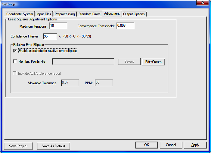
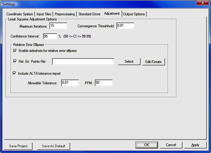
Maximum Iterations: Non-linear least
squares is an iterative process. The user must define the maximum number
of iterations to make before the program quits trying to find a converging
solution. Typically if there are no blunders in the data the solution will
converge in 2-5 iterations.
Convergence Threshold: During each iteration corrections are computed. When the corrections are less than the threshold value the solution has converged. This value should be somewhat less than the accuracy of the measurements. For example, if you can only measure distances to the nearest .01' then a reasonable convergence threshold value would be .005'.
Confidence Interval: This setting is used when calculating the size of error ellipses, and in the chi-square testing. For example, a 95% confidence interval means that there is a 95% chance that the error is within the tolerances shown.
Enable sideshots for relative error ellipses: Check this box if you want to see the error ellipses and relative error ellipses of sideshots. This checkbox must be set if you want to use the relative error ellipse inverse function with sideshots. When turned off this toggle filters out sideshots during the least squares processing. Since the sideshots are excluded form the least squares processing error ellipses cannot be computed for these points. When this toggle is off, the sideshots are computed after the network has been adjusted. The final coordinate values of the sideshots will be the same regardless of this setting.
Large numbers of sideshots slow down least squares processing. It is best to uncheck this box while debugging your project to avoid having to wait for the computer to finish processing. After the project processes correctly you may turn on the option for the final processing.
Relative Err. Points File: The new ALTA standards require that surveyors certify to the relative positional error between points. Relative error ellipses are an accepted method of determining the relative positional error required by the ALTA standards. The points that are to be included in the relative error checking are specified by the user. These points are defined in an ASCII file with an extension of .ALT. To select an .alt file for relative error checking use the [Select] button and then browse to the file's location.
Include ALTA
tolerance report: Turn this toggle on if you wish to include the ALTA
tolerance section of the report.
Allowable Tolerance, PPM: These fields allow the user to set the
allowable error for computations. Typically the user would enter the current
ALTA error standards, i.e. 0.07' & 50 PPM.
See the ALTA section later in this manual for more detailed information on creating and interpreting the ALTA section of the report.
Standard Errors
Standard errors are the expected measurement errors based on the type equipment and field procedures being used. For example, if you are using a 5 second total station, you would expect the angles to be measured within +/- 5 seconds (Reading error).
The Distance Constant, PPM settings, and Angle Reading
should be based on the equipment and field procedures being used. These
values can be obtained from the published specifications for the total station,
or the distance PPM and constant can be computed for a specific EDM by
performing an EDM calibration using an EDM calibration baseline.
Survey methods should also be taken into account when setting standard errors. For example, you might set the target centering standard error higher when you are sighting a held prism pole than you would if you were sighting a prism set on a tripod.
The settings from this dialog box will be used for the project default settings. These default standard errors can be overridden for specific measurements by placing SE records directly into the Raw Data File (see the above section on raw data files).
If the report generated when you process the data shows that generally you have consistently high standard residuals for a particular measurement value (angles, distances, etc.), then there is the chance that you have selected standard errors that are better than your instrument and methods can obtain. (See explanation of report file). Failing the chi-square test consistently is also an indication that the selected standard errors are not consistent with the field measurements.
You can set the standard errors for the following:
Distance and Angle Standard Errors
Distance Constant: Constant portion of the distance error. This value can be obtained from published EDM specifications, or from an EDM calibration.
Distance PPM: Parts per million component of the distance error. This value can be obtained from published EDM specification, or from an EDM calibration.
Horizontal Angle Pointing: The horizontal angle pointing error is influenced by atmospheric conditions, optics, experience and care taken by instrument operator.
Horizontal Angle Reading: Precision of horizontal angle measurements, obtain from theodolite specs.
Vertical Angle Pointing: The vertical angle pointing error is influenced by atmospheric conditions, optics, experience and care taken by instrument operator.
Vertical Angle Reading: Precision of vertical angle measurements, obtain from theodolite specs.
Instrument and Target Standard Errors
Target Centering: This value is the expected amount of error in setting the target or prism over the point.
Instrument Centering: The expected amount of error in setting the total station over the point.
Target Height: The expected amount of error in measuring the height of the target.
Instrument Height: The expected amount of error in measuring the height of the total station.
Control Standard Errors
Direction (Bearing / Azimuth): The
estimated amount of error in the bearing/azimuth (direction) found in the
azimuth records of the raw data.
North, East, Elev: The estimated amount of error in the control
north, east and elev. You may want to have different coordinate standard
errors for different methods of obtaining control. Control derived from
RTK GPS would be higher than control derived from GPS static measurements.
GPS Standard Errors
Instrument Centering: This option is used to specify the error associated with centering a GPS receiver over a point.
Vector Standard Error Factor: This option is used as a factor to increase GPS vector standard errors as found in the input GPS vector file. Some people think that the GPS vector variances/covariances as found in GPS vector files tend do be overly optimistic. This factor allows the user to globally increase the GPS vector standard errors without having to edit the GPS vector file. A factor of 0 should be the default value and results in no change to the GPS vector standard errors as found in the GPS vector file. The maximum value allowed is 10.
Differential Leveling Standard Errors
These settings only effect level data and are not used when processing total station or GPS vector files.
Avg, Dist. To BS/FS: This option is used to define the average distance to the backsight and foresight during leveling.
Rod Reading Error per 100 ft./m: This option is used to define the expected level reading error.
Collimation Error: This is the expected differential leveling collimation error in seconds.
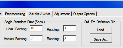
Standard Error Definition Files
The Standard Error settings can be saved and then later reloaded into an existing or new project. Creating libraries of standard errors for different types of survey equipment or survey procedures is a convenient method of creating standards within a survey department using a variety of equipment and performing different types of surveys. Standard error library files, *.SEF files, can be created two ways. From the Settings/Standard Errors dialog box the [Load] button can be used to import an existing .SEF file into the current project. A .SEF file can also be created from the existing project standard errors by using the [Save As] button.
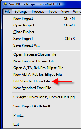
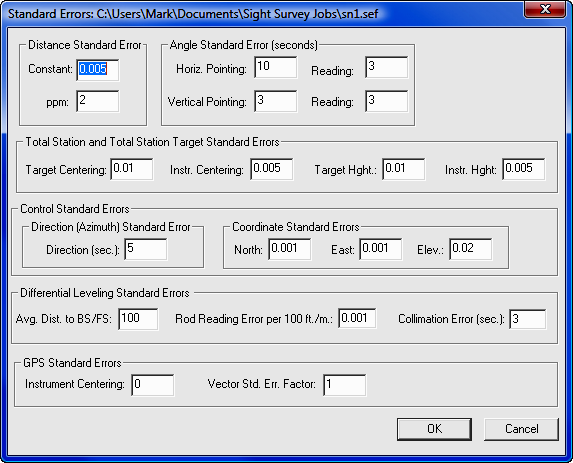
Standard error files (.SEF) can also be managed from the main Files menu. Use the Edit Standard Error File menu option to edit an existing standard error file. Use the New Standard Error File option to create a new standard error file.
After choosing one of the menu options and choosing the file to edit or create, the following dialog box will be shown. Set the desired standard errors and press the [OK] button to save the standard error file.
These settings apply to the output of data to the report and coordinate files.
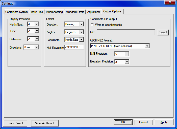
These settings determine the number of decimal places to display in the reports for the following types of data. The display precision has no effect on any computations, only the display of the reports.
Coordinates (North, East, Elevation) - Chose 0-4 decimal places.
Distances - Chose 0-4 decimal places
Directions (Azimuths or Bearings) - nearest second, tenth of second, or
hundredth of second.
These settings determine the format for the following types of data.
Direction - Choose either bearings or azimuth for direction display. If the angle units are degrees, bearings are entered as QDD.MMSSss and azimuths are entered as DDD.MMSSss. If the angle units are grads, bearings are input as QGGG.ggggg and azimuths are input as GGG.ggggg.
Coordinate Display - Choose the order of coordinate display, either north-east or east-north.
Null Elevation - Choose the value for null elevations in the output ASCII coordinate NEZ file. The Null Elevation field defaults to SurvNET’s value for NO ELEVATION,of -999999999.0 .
Angle Display - Choose the units you are working it: degrees; or gradians.
Coordinate File Output
These settings determine the type and format of the output NEZ file. An ASCII .NEZ and .OUT files are always created after processing the raw data. The .OUT file will be a nicely formatted version of the .NEZ file suitable for printing. The .NEZ file will be an ASCII file suitable to be input into other programs. There are a variety of options for the format of the .NEZ file. Following are the different ASCII file output options.
P,N,E,Z,CD,DESC (fixed columns); - Point,north,east,elev.,code,desc in fixed columns separated by commas.
P,N,E,Z,CD,DESC; Point,north,east,elev.,code,desc separated by commas.
P N E Z CD DESC (fixed columns); Point,north,east,elev.,code,desc in fixed columns with no commas.
P N E Z CD DESC; Point,north,east,elev.,code,desc in fixed columns with no commas.
P,N,E,Z,DESC (fixed columns); Point,north,east,elev., desc in fixed columns separated by commas.
P,N,E,Z,DESC; Point,north,east,elev., desc separated by commas.
P N E Z DESC (fixed columns); Point,north,east,elev., desc in fixed columns with no commas.
P N E Z DESC; Point,north,east,elev.,code,desc separated by spaces.
P,E,N,Z,CD,DESC (fixed columns); - Point,east,north,elev.,code,desc in fixed columns separated by commas.
P,E,N,Z,CD,DESC; Point,east,north,elev.,code,desc separated by commas.
P E N Z CD DESC (fixed columns); Point,east,north,elev.,code,desc in fixed columns with no commas.
P E N Z CD DESC; Point,east,north,elev.,code,desc in fixed columns with no commas.
P,E,N,Z,DESC (fixed columns); Point,east,north,elev., desc in fixed columns separated by commas.
P,E,N,Z,DESC; Point,east,north,elev., desc separated by commas.
P E N Z DESC (fixed columns); Point,east,,northelev., desc in fixed columns with no commas.
P E N Z DESC; Point,east,north,elev.,code,desc separated by spaces.
CSV ASCII with std. errors (This format is useful as it can be used as a supplemental control input file type option, where the coordinate standard errors output for one project can be used as input for another project.)
You can also set the output precision of the coordinates for the ASCII output file. This setting only applies to ASCII files, not to the C&G or Carlson binary coordinate files which are stored to full double precision.
N/E Precision: number of places after the decimal to use for North and East values (0 -> 8) in the output NEZ ASCII file.
Elevation Precision: number of places after the decimal to use for Elevation values (0 -> 8) in the output NEZ ASCII file.
If you want to write the calculated coordinates directly to a coordinate file,
check the Write to Carlson/C&G .CRD file box and select the file.
You can choose the type of Carlson/C&G file to be created when you select the
file to be created. You may wish to leave this box unchecked until you are
satisfied with the adjustment. Following are the different available
coordinate output file options.
C&G Numeric (.crd)
C&G Alphanumeric (.cgc)
Carlson Numeric (.crd)
Carlson Alphanumeric (.crd)
Autodesk Land Desktop (.mdb)
Simplicity (.zak)
NOTE: If coordinate points already exist in the CRD file, before a point is written, you will be shown the NEW value, the OLD value, and given the following option:
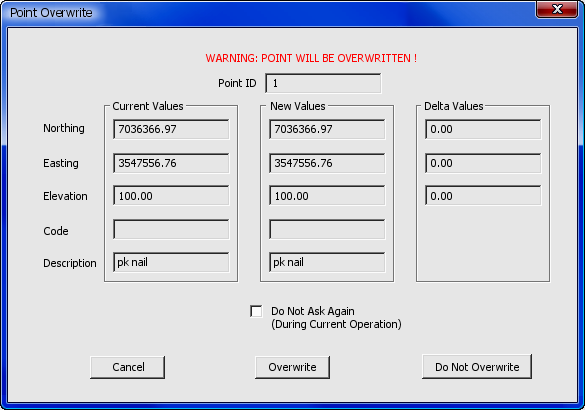
Cancel: Cancel the present operation. No more points will be written to the Carson/C&G file.
Overwrite: Overwrite the existing point. Notice that if you check the Do Not Ask Again box all further duplicate points will be overwritten without prompting.
Do not Overwrite: The existing point will not be overwritten. Notice that if you check the Do Not Ask Again box all further duplicate points will automatically not be overwritten and only new points will be written.
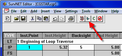
When you select Process > Network Adjustment from the menu, or select the NETWORK icon on the tool bar, the raw data will be processed and adjusted using least squares based on the project settings. If there is a problem with the reduction, you will be shown error messages that will help you track down the problem. Additionally an .err file is created that will log and display error and warning messages.
The data is first preprocessed to calculate averaged angles and distances for sets of angles and multiple distances. For a given setup, all multiple angles and distances to a point will be averaged prior to the adjustment. The standard error as set in the Project Settings dialog box is the standard error for a single measurement. Since the average of multiple measurements is more precise than a single measurement the standard error for the averaged measurement is computed using the standard deviation of the mean formula.
Non-linear network least squares solutions require that initial approximations of all the coordinates be known before the least squares processing can be performed. During the preprocessing approximate coordinate values for each point are calculated using basic coordinate geometry functions. If there is inadequate control or odd geometric situations SurvNET may generate a message indicating that the initial coordinate approximations could not be computed. The most common cause of this problem is that control has not been adequately defined or there are point number problems.
Side Shots are separated from the raw data and computed after the adjustment (unless the Enable sideshots for relative error ellipses toggle is checked in the adjustment dialog box). If side shots are filtered out of the least squares process and processed after the network is adjusted, processing is greatly speeded up, especially for a large project with a lot of side shots.
If the raw data processes completely, a report file, .RPT, a .NEZ file, an .OUT file, and an .ERR file will be created in the project directory. The file names will consist of the project name plus the above file extensions. These different files are shown in separate windows after processing. Additionally a graphic window of the network is displayed.
.RPT file: This is an ASCII file that contains the statistical and computational results of the least squares processing.
.NEZ file: This file is an ASCII file containing the final adjusted coordinates. This file can be imported into any program that can read ASCII coordinate files. The format of the file is determined by the setting in the project settings dialog box.
.OUT file: The .OUT file is a formatted ASCII file of the final adjusted coordinates suitable for display or printing
.ERR file: The .ERR file contains any warning or error messages that were generated during processing. Though some warning messages may be innocuous it is always prudent to review and understand the meaning of the messages.
The following is a graphic of the different windows displayed after processing. Notice that with the report file you can navigate to different sections of the report using the tabs at the top of the window.
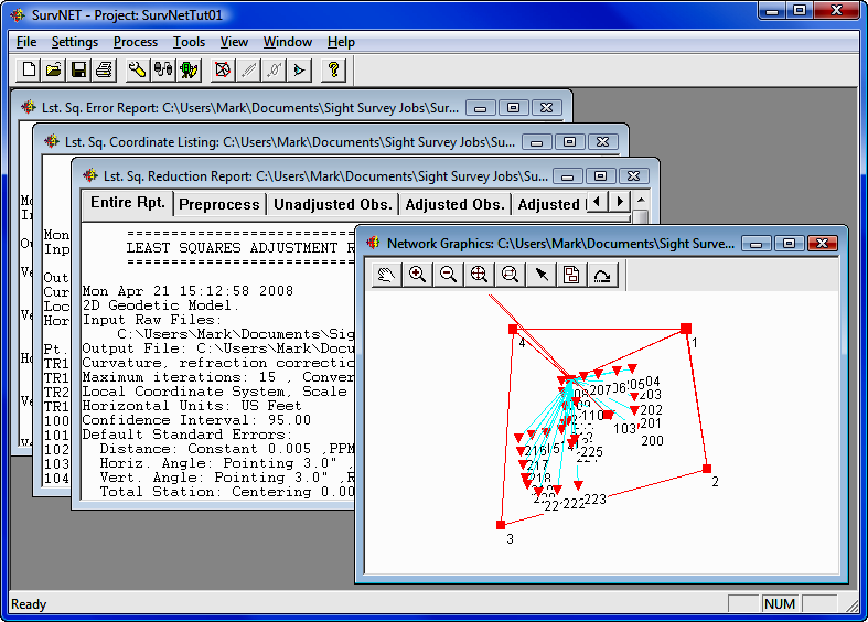
If you have Write to Carlson/C&G.CRD checked in the output options dialog, the coordinates will also be written to a .CRD file.
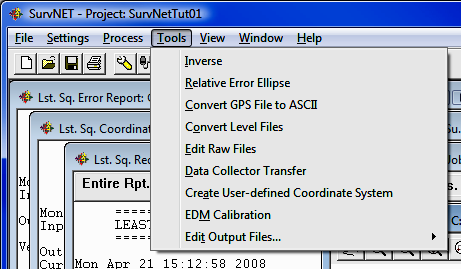
Inverse
Button - The Inverse button is found on the
main window (the button with the icon that shows a line with points at each
end). You can also select the Tools > Inverse menu option.
This feature is only active after a network has been processed successfully.
This option can be used to obtain the bearing and distance between any two
points in the network. Additionally, the standard deviation of the bearing
and distance between the two points is displayed.
The Relative Error Ellipse Inverse button is found on the main window
(the button with the icon that shows a line with an ellipse in the middle).
You can also select the Tools > Relative Error Ellipse menu option.
This feature is only active after a network has been processed successfully.
This option can be used to obtain the relative error ellipse between two points.
It shows the semi-major and semi-minor axis and the azimuth of the error
ellipse, computed to a user-define confidence interval. This information
can also be used to determine the relative precision between any two points in
the network. It is the relative error ellipse calculation that is the
basis for the ALTA tolerance reporting. If the Enable sideshots for
relative error ellipses toggle is checked, all points in the project can be
used to compute relative error ellipses. The trade-off is that processing
time will be increased with large projects.
If you need to certify as to the Positional Tolerances of your monuments as per the ALTA Standards, use the Relative Error Ellipse Inverse routine to determine these values, or use the specific ALTA tolerance reporting function as explained later in the manual.
For example, suppose you must certify that all monuments have a positional tolerance of no more than 0.07 feet with 50 PPM at a 95 percent confidence interval. First set the confidence interval to 95 percent in the Settings/Adjustment screen, then process the raw data. Now you may inverse between points in as many combinations as you deem necessary and make note of the semi-major axis error values. If none of them are larger than 0.07 feet + (50PPM*distance), you have met the standards. It is however more convenient to create a Relative Error Points File containing the points you wish to check and include the ALTA tolerance report. This report takes into account the PPM and directly tells you if the positional tolerance between the selected points meets the ALTA standards.
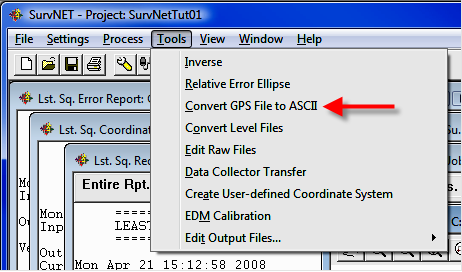
The purpose of this option is to convert GPS vector files that are in the manufacturers' binary or ASCII format into the StarNet ASCII file format. The advantage of creating an ASCII file is that the ASCII file can be edited using a standard text editor. Being able to edit the vector file may be necessary in order to edit point numbers so that the point numbers in the GPS file match the point numbers in the total station file. The following dialog box is displayed after choosing this option.
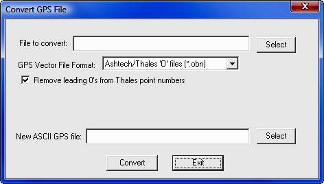
First choose the file format of the GPS vector file to be converted. Next use the [Select] button to navigate to the vector file to be converted. If you are converting a Thales file you have the option to remove the leading 0's from Thales point numbers. Next, use the second [Select] button to select the name of the new ASCII GPS vector file to be created. Choose the [Convert] button to initiate the file conversion. Press the [Cancel] button when you have completed the conversions. The file created will have an extension of .GPS. Following are the different GPS formats that can be converted to ASCII.
Thales: The Thales GPS vector file is a binary file and is sometimes referred to as an 'O' file. Notice that you have the option to remove the leading 0's from Thales point numbers, by checking the Remove leading 0's from Thales point numbers check box.
Leica: The Leica vector file is an ASCII format typically created with the Leica SKI software. This format is created by Leica when baseline vectors are required for input into 3rd party adjustment software such as SurvNET. The SKI ASCII Baseline Vector format is an extension of the SKI ASCII Point Coordinate format.
Topcon (.TVF): The Topcon Vector File is in ASCII format and typically has an extension of .TVF
Topcon (.XML): The Topcon XML file is an ASCII file that contains the GPS vectors in an XML format. This format is not equivalent to LandXML format.
Trimble Data Exchange Format (.ASC): The Trimble TDEF format is an ASCII file typically output by Trimble's office software as a means to output GPS vectors for use by 3rd party software.
Trimble Data Collection (.dc): The Trimble .dc format is an ASCII file typically output by Trimble's data collector. It contains a variety of measurements including GPS vectors. This option only converts GPS vectors found in the .DC file.
LandXML (.XML): The landXML format is an industry standard format. Currently SurvNET will only import LandXML survey point records. The conversion does not currently import LandXML vectors.
NGS G-File: The NGS G-File is the format used National Geodetic Survey in their processing software.
NGS G-File from an OPUS report: Every OPUS report contains a G-File section. The vectors making up this G-file are the vectors from the control points to the computed point making up the OPUS solution. These OPUS vectors can be extracted and then combined with other GPS or total station data to create a larger SurvNET project. If the OPUS vector data is used in a SurvNET project it is important to use Geoid modeling since the control points making up the OPUS solution typically cover a large extents.
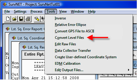
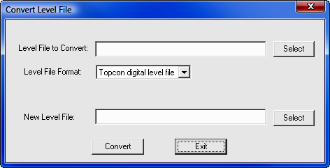
The purpose of this option is to convert differential level files from digital levels into C&G/Carlson differential level file format. At present the only level file format that can be converted are the level files downloaded from the Topcon digital levels.
Select Edit Raw Files to open a raw file editor. If you are using a C&G raw file (.CGR), the C&G Raw Editor will open. Please refer to see Section 11.10 for instructions on the C&G Raw Editor. If you are using a Carlson raw file (.RW5), the Carlson Raw Editor will open. Please refer to see Section 11.11 for instructions on the Carlson Raw Editor.
Select Data Collector Transfer to open a data transfer program. If you are using C&G data files, the C&G Transfer program will open. Please refer to see Section 11.08 for instructions on using C&G Transfer. If you are using Carlson data files, the Carlson SurvCom program will open. Please refer to see Section 11.09 for instructions on using SurvCom.
The EDM Calibration program allows a surveyor to
enter and process the raw data collected on an EDM calibration baseline.
The purpose of an EDM calibration is to determine if the EDM is measuring within
standards. The program performs a statistical analysis of that data as outlined
in "Use of Calibration Base Lines", by Charles J. Fronczek, NOAA Technical
Memorandum NOS NGS-10. The NGS document can be downloaded from the NGS
website. NGS maintains a webpage on EDM Calibration Base Lines. The
manual and other information on EDM calibrations can be found at
http://geodesy.noaa.gov/CBLINES/calibration.shtm. Following is
the main EDM Calibration dialog box. NGS publishes the EDM
calibration data in metric units. SurvNET's EDM calibration program
currently expects the data to be collected in meters.
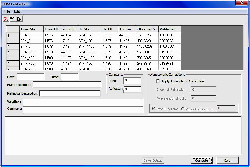
The basic flow of this program is to first fill out the lower portion of the
dialog box which contains different text fields, EDM constant values, and
the optional Atmospheric Corrections settings. Next, fill out the
grid in the upper portion of the dialog box. This grid contains the field
data collected and also the published distances between monuments of the
baseline. After this information has been filled out use the [Compute]
button. The program will then display the result of the calibration in the
window in the lower portion of the dialog box as follows.
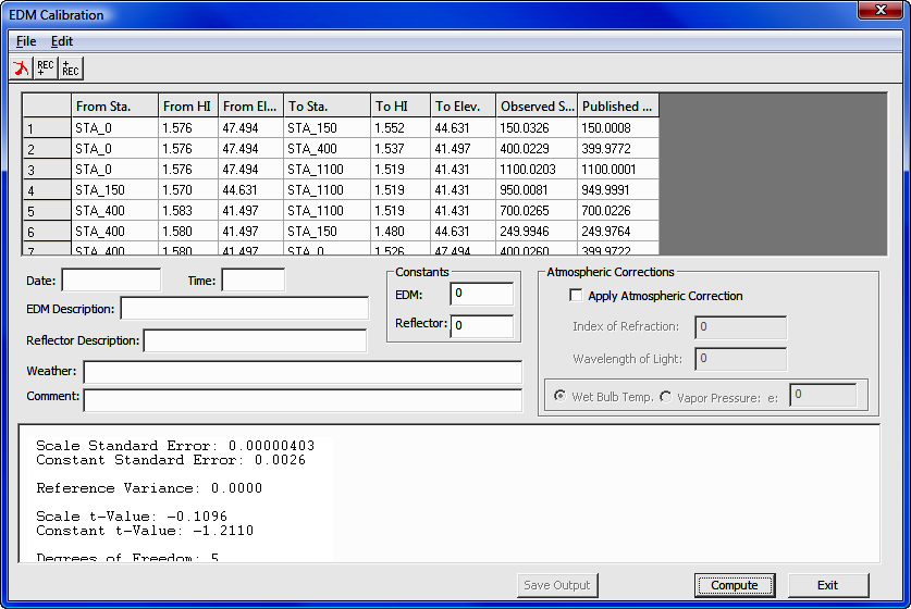
After the file is processed the results can be stored as an ASCII text file.
Use the [Save Output] button or the menu
option File > Save Results File As to save the results. First, you
will be prompted for an output file name. The input data can also be
stored. Once stored it can be opened and processed again.
Following is the entire output with a brief explanation of the results. Comments about the results are inserted between report sections.
EDM Calibration Report
Observed Data
EDM Type:
Date: Time:
Prism description:
Weather description:
Comment:
Atmosphere Correction: OFF
Constants: Refrector: 0.000 EDM: 0.000
From From From To . To To Observed Published
Sta. Elev. HI Sta. Elev. HI Temp. Pressure Slope Dist. Dist.
STA_0 47.494 1.576 STA_150 44.631 1.552 0.0 0.0 150.0326 150.0008
STA_0 47.494 1.576 STA_400 41.497 1.537 0.0 0.0 400.0229 399.9772
STA_0 47.494 1.576 STA_1100 41.431 1.519 0.0 0.0 1100.0203 1100.0001
STA_150 44.631 1.570 STA_1100 41.431 1.519 0.0 0.0 950.0081 949.9991
STA_400 41.497 1.583 STA_1100 41.431 1.519 0.0 0.0 700.0265 700.0226
STA_400 41.497 1.580 STA_150 44.631 1.480 0.0 0.0 249.9946 249.9764
STA_400 41.497 1.580 STA_0 47.494 1.526 0.0 0.0 400.0260 399.9722
The above section shows the inputs, which consists of the observed slope distances and the measured HI's. The From and To elevations are published data from the NGS data sheet on the particular baseline being observed. The published distances are also published NGS data sheet. In this example, the atmospheric pressure was turned OFF so the Temperature and Pressure fields are irrelevant.
Results
Null Hypothesis, HO: EDM scale error and EDM constant error = 0.0
If the scale error and the EDM constant are 0.0 then the EDM is without error. So the purpose of the statistical test is to test how close the results are to 0.0.
Scale Error (ppm): -0.00000044
Constant Error: -0.0032
The two above lines show the values for the
computed scale error and constant error.
Scale Standard Error: 0.00000403
Constant Standard Error: 0.0026
The two above lines show the values for the computed standard errors of the scale error and constant error.
Reference Variance: 0.0000126
Scale t-Value: -0.1096
Constant t-Value: -1.2110
Degrees of Freedom: 5
Critical t-Value at the 1 percent confidence level: 4.0320
Cannot reject the H0 for the scale error. (The scale factor is 0.0)
Cannot reject the H0 for the constant error. (The constant is 0.0)
The above lines show the final results of the statistical test.  Since the test determined that we cannot reject the
null hypothesis, this EDM is in good working order.
The atmospheric correction algorithms used in the EDM calibration are from the NGS manual. To use this method both dry-bulb and wet-bulb temperature needs to be measured; or the vapor pressure, e, and the dry bulb temperature needs to be measured. Refer to the NGS documentation for a detailed explanation of the atmospheric corrections that they use.
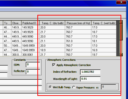
It is probably most common to turn atmospheric correction
OFF in
the calibration program, and turn atmospheric correction
ON on the EDM (total
station). When atmospheric correction is turned off in the calibration
program the user does not need to enter the temperature into the grid or any of
the other atmospheric values. If atmospheric corrections are turned
OFF
then the grid input columns Temp.(dry bulb), Pressure, (mm of Hg),
and Temp. (wet bulb) will not be displayed since they are not needed.
Constants can be entered for both the EDM and the reflector. These values
are added to the observed distances during processing. Typically they are
set to 0.0.
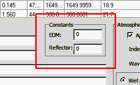
The following text fields have no effect on any computations and
are simply comments that can be used to document the calibration.
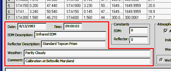
Blank data records are inserted into or deleted from the grid using the following tool bar.
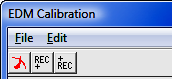
The first button deletes the current highlighted record. The second
button inserts a new blank record before the current highlighted record. The
third button inserts a new blank record after the current highlighted record.
Alternately the Edit menu options could be used to delete and insert
new data records.
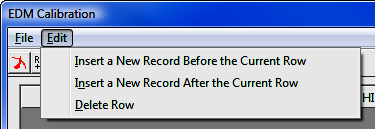
Following is a brief explanation of the fields that make up the grid.
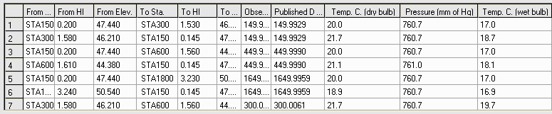
From Sta. - This field represents the station name where the EDM is
located. Any name can be used, but you must be consistent and used the same name
whenever you occupy or measure a distance to the station.
From HI. - This field represents the height of instrument of the from
station. It should be in the same units as the measurements. If
horizontal distances are being entered into the grid then all the HI fields
should be set to a constant value such as 0.0.
From Elev. - This field represents the elevation of the station. This
value is published as part of the baseline calibration sheets obtained from NGS.
If horizontal distances are used then all the Elevation fields should be set to
a constant.
To Sta. - This field represents the
station name where the prism is located. Any name can be used but you must
be consistent and use the same name whenever you occupy or measure a distance to
the station.
To HI. - This field represents the height of instrument of the to station.
It should be in the same units as the distance measurements. If horizontal
distances are being entered into the grid then all the HI fields can be set to a
constant value such as 0.0.
To Elev. - This field represents the elevation of the station where the
prism is located. This value is published as part of the baseline
calibration sheets obtained from NGS. If horizontal distances are used
then all the Elevation fields should be set to a constant.
Observed S. Dist. - This is the measured slope distance or it can be a
measured horizontal distance. If it is a horizontal distance then all the
HI's and elevations should be set to a constant value.
Published Dist. - This field represents the published distance between the
From and To station. This value is published as part of the
baseline calibration data obtained from NGS for the particular baseline being
observed.
Temp. (dry bulb) - This field is only present if atmospheric corrections are
turned on.
Temp. (wet bulb) - This field is only present if atmospheric corrections are
turned on.
Pressure. (mm of Hg) - This field is only present if atmospheric corrections
are turned on.
Many of the most commonly used functions can be accessed using the toolbar. Following is an explanation of the buttons found in the toolbar.
![]()
|
|
Create New Project - New project icon. |
|
|
Open an Existing Project - Open file icon. |
|
|
Save the Current Project - Disk icon. |
|
|
Print One of the Reports - Printer icon. |
|
|
Settings -Wrench icon. This icon initiates the Settings > Standard Errors tab. |
|
|
Data Collector Transfer Program - This icon will initiate either the C&G Data Transfer program or the Carlson SurvCom program. The C&G program allows you to transfer data from the data collector, or convert the data collector file to a .CGR file format. It supports all major data collectors. The Carlson program connects specifically to the Carlson SurvCE data collector. |
|
|
Edit Raw Data - This icon can be used to start either the .RW5 raw data editor or the .CGR raw data editor. If your project has multiple raw data files, you will be shown a list and asked to select the file you wish to edit. The appropriate editor will be called depending on what type raw files are defined in the project settings. If no raw file or project has been specified the default raw editor as defined in the Settings menu will be executed. Any changes you make in the editor need to be saved before returning to SurvNET for processing. |
|
|
Process Network - Icon that looks like a traverse network. |
|
|
Inverse - Icon has a line with points on each end. |
|
|
Relative Error Ellipses - Icon has a line with points on each end and an ellipse in the middle |
|
|
Graphics - Icon that looks like an eye. This icon is active once a project has been opened. |
|
|
Help - Question mark icon. |
Report
File: A report file consisting of the project
name with an .RPT extension is generated after successfully processing the raw
data. The report file will be shown in a text window so you can analyze
the data. You can pick the Printer icon if you wish to produce a
hardcopy. Following is an example of the results from a relatively simple
network adjustment using a local coordinate system.
Sample 2D/1D, Local Coordinate System
Report File
================================
LEAST SQUARES ADJUSTMENT REPORT
================================
Mon May 08 10:16:16 2006

2D Geodetic Model.

Input Raw Files:
    C:\data\lsdata\cgstar\CGSTAR.CGR
Output File: C:\data\lsdata\cgstar\cgstar.RPT

Curvature, refraction correction: ON

Maximum iterations: 10 , Convergence Limit: 0.002000
Local Coordinate System, Scale Factor: 1.000000
Horizontal Units: US Feet
Confidence Interval: 95.00

Default Standard Errors:
Distance: Constant 0.010 ,PPM: 5.000
Horiz. Angle: Pointing 3.0" ,Reading: 3.0"
Vert. Angle: Pointing 3.0" ,Reading: 3.0"
Total Station: Centering 0.005 ,Height: 0.010
Target: Centering 0.005 ,Height: 0.010
Azimuth: 5"

Coordinate Control: N:0.010, E:0.010, Z:0.030,


Horizontal Angle spread exceeds tolerance:
  IP: 1,  BS: 5,  FS: 2
  Low: 109-19'10.0" ,  High: 109-19'17.0" ,  Diff: 000-00'07.0"

Horizontal Angle spread exceeds tolerance:
  IP: 2,  BS: 1,  FS: 6
  Low: 190-32'02.0" ,  High: 190-32'10.0" ,  Diff: 000-00'08.0"
Horizontal Angle spread exceeds tolerance:
  IP: 2,  BS: 1,  FS: 3
  Low: 096-03'48.0" ,  High: 096-03'56.0" ,  Diff: 000-00'08.0"
Horizontal Angle spread exceeds tolerance:
  IP: 3,  BS: 2,  FS: 4
  Low: 124-03'50.0" ,  High: 124-03'56.0" ,  Diff: 000-00'06.0"

Horizontal Angle spread exceeds tolerance:
  IP: 5,  BS: 4,  FS: 10
  Low: 039-26'35.0" ,  High: 039-26'45.0" ,  Diff: 000-00'10.0"
Horizontal Angle spread exceeds tolerance:
  IP: 10,  BS: 5,  FS: 11
  Low: 241-56'23.0" ,  High: 241-56'35.0" ,  Diff: 000-00'12.0"
Horizontal Angle spread exceeds tolerance:
  IP: 11,  BS: 10,  FS: 12
  Low: 114-56'20.0" ,  High: 114-56'34.0" ,  Diff: 000-00'14.0"
Horizontal Angle spread exceeds tolerance:
  IP: 12,  BS: 11,  FS: 3
  Low: 140-39'18.0" ,  High: 140-39'31.0" ,  Diff: 000-00'13.0"

Horizontal Angle spread exceeds tolerance:
  IP: 5,  BS: 4,  FS: 1
  Low: 117-30'35.0" ,  High: 117-30'50.0" ,  Diff: 000-00'15.0"

Horizontal Distance from 2 to 3 exceeds tolerance:
  Low: 324.15,  High: 324.20,  Diff: 0.04

Vertical Distance from 2 to 3 exceeds tolerance:
  Low: 6.62,  High: 8.36,  Diff: 1.74
Vertical Distance from 3 to 4 exceeds tolerance:
  Low: 11.46,  High: 11.51,  Diff: 0.05

Horizontal Distance from 12 to 3 exceeds tolerance:
  Low: 144.64,  High: 144.66,  Diff: 0.02


     HORIZONTAL ADJUSTMENT REPORT
     ============================
Unadjusted Observations
=======================


Control Coordinates:     1 Observed Points,    0 Fixed Points,    0 Approx. Points

Sta.            N:            E:           StErr N:   StErr E:

1              658428.26    2150182.70       0.01        0.01


Distances:   14 Observations

From Sta.   To Sta.               Dist.       StErr

1             5                  290.45        0.01
1             2                  292.21        0.01
2             6                   52.39        0.01
2             3                  324.19        0.01
3             4                  275.60        0.01
3             20                 134.66        0.01
20            21                 116.07        0.01
21            22                  50.12        0.01
4             5                  309.65        0.01
5             10                 129.99        0.01
10            11                 126.01        0.01
10            15                  10.00        0.01
11            12                 129.43        0.01
12            3                  144.65        0.01


Angles:   15 Observations

BS Sta.  Occ. Sta.   FS Sta.         Angle         StErr (Sec.)

5          1           2          109-19'13.5"          7.7
1          2           6          190-32'06.0"         26.2
1          2           3          096-03'52.0"          7.3
2          3           4          124-03'53.0"          7.8
2          3           20         185-23'56.0"         12.8
3          20          21         180-15'26.0"         17.6
20         21          22         183-26'45.0"         31.2
3          4           5          093-02'11.5"          7.5
4          5           10         039-26'40.0"         10.4
5          10          11         241-56'29.0"         15.6
5          10          15         056-23'10.0"        125.0
10         11          12         114-56'27.0"         15.5
11         12          3          140-39'24.5"         15.3
12         3           2          325-54'30.0"          9.5
4          5           1          117-30'42.5"          7.7


Azimuths:    1 Observations

Occ. Sta.   FS Sta.       Bearing        StErr (Sec.)

1            2          N 45-00'00.0"E        5.0


Adjusted Coordinates
====================


Adjusted Local Coordinates

Sta.            N:            E:           StErr N:   StErr E:

1              658428.26    2150182.70       0.02       0.02
2              658634.88    2150389.32       0.02       0.02
5              658554.12    2149920.92       0.03       0.02
3              658887.03    2150185.59       0.02       0.03
4              658863.61    2149910.99       0.03       0.03
20             658999.28    2150111.19       0.03       0.04
21             659096.31    2150047.49       0.04       0.05
10             658657.11    2150000.25       0.03       0.03
11             658636.21    2150124.52       0.03       0.03
12             658742.89    2150197.81       0.03       0.03


Adjusted Coordinates Error Ellipses, 95% CI

Sta.               Semi Major      Semi Minor        Max. Error Az.
                      Axis            Axis

1                      0.05            0.05          S 29-26'39.4"E
2                      0.07            0.07          N 45-00'00.0"E
5                      0.08            0.07          N 10-58'28.2"E
3                      0.10            0.07          N 84-37'31.0"E
4                      0.11            0.07          N 51-23'12.0"E
20                     0.13            0.10          N 84-24'17.5"E
21                     0.17            0.12          N 72-01'17.5"E
10                     0.09            0.07          N 43-35'54.5"E
11                     0.09            0.08          N 54-43'51.1"E
12                     0.08            0.08          N 79-48'07.2"E


Adjusted Observations
=====================


Adjusted Distances

From Sta.  To Sta.        Distance    Residual     StdRes.   StdDev

1             5             290.46      0.01          1.42     0.01
1             2             292.21     -0.00          0.40     0.01
2             3             324.17     -0.01          1.62     0.01
3             4             275.59     -0.01          1.11     0.01
3             20            134.66     -0.00          0.00     0.02
20            21            116.07     -0.00          0.00     0.02
4             5             309.65      0.01          0.64     0.01
5             10            130.00      0.01          0.97     0.01
10            11            126.01      0.00          0.16     0.01
11            12            129.44      0.01          0.98     0.02
12            3             144.66      0.01          0.94     0.02

           Root Mean Square (RMS)       0.01


Adjusted Angles

BS Sta.  Occ. Sta.   FS Sta.       Angle          Residual     StdRes   StdDev(Sec.)

5           1          2        109-19'19.2"        5.7         0.7         9.9
1           2          3        096-03'43.4"       -8.6         1.2         9.2
2           3          4        124-03'48.1"       -4.9         0.6        10.1
2           3          20       185-23'56.0"       -0.0         0.0        21.5
3           20         21       180-15'26.0"        0.0         0.0        29.7
3           4          5        093-02'12.8"        1.3         0.2         9.3
4           5          10       039-26'37.1"       -2.9         0.3        14.4
5           10         11       241-56'27.5"       -1.5         0.1        21.2
10          11         12       114-56'39.8"       12.8         0.8        21.8
11          12         3        140-39'40.8"       16.3         1.1        20.3
12          3          2        325-54'33.8"        3.8         0.4        13.2
4           5          1        117-30'56.6"       14.1         1.8         9.9

                     Root Mean Square (RMS)         8.1


Adjusted Azimuths

Occ. Sta.  FS Sta.      Bearing           Residual       StdRes    StdDev(Sec.)

1           2          N 45-00'00.0"E        0.0           0.0          8.4

               Root Mean Square (RMS)        0.0


Statistics
==========

Solution converged in 2 iterations
Degrees of freedom:6
Reference variance:2.84
Standard error unit Weight: +/-1.68
Failed the Chi-Square test at the 95.00 significance level
1.237 <= 17.023 <= 14.449


Sideshots
=========


From  To         Bearing         Dist.      N             E    StDev. N  StDev. E


2     6       N 55-32'06.0"E     52.39    658664.53   2150432.52    0.02    0.02
21    22      N 29-50'09.6"W     50.12    659139.78   2150022.56    0.04    0.05
10    15      N 86-00'28.6"W     10.00    658657.80   2149990.27    0.03    0.03


                 LEAST SQUARES VERTICAL ADJUSTMENT REPORT


Mon May 08 10:16:16 2006

2D Geodetic Model.

Input Raw Files:
    C:\data\lsdata\cgstar\CGSTAR.CGR
Output File: C:\data\lsdata\cgstar\cgstar.RPT

Curvature, refraction correction: ON


                            FIXED VERTICAL BENCHMARKS


Station            Elevation

1                   569.8500


                            POINTS TO BE ADJUSTED

Station
2,5,3,4,10,11,12


                                MEASUREMENT SUMMARY


From          To           Elev. Diff.
                          (unadjusted)      StdErr

1             5                 7.5040      0.0145
1             2                 7.5659      0.0145
2             3                 6.9843      0.0145
3             4               -11.4907      0.0146
4             5                 4.3557      0.0145
5             10                2.2639      0.0143
10            11                1.0931      0.0143
11            12                0.3828      0.0143
12            3                 3.3590      0.0144


                              ADJUSTED ELEVATIONS


Station     Adjusted Elev   Standard Dev.

1               569.8500        0.00000
2               577.4336        0.02465
5               577.3363        0.02465
3               584.4355        0.02915
4               572.9628        0.03070
10              579.6003        0.03341
11              580.6935        0.03641
12              581.0764        0.03519


                        ADJUSTED MEASUREMENT SUMMARY


From        To            Elev. Diff.      Residuals
                           (adjusted)

1            5                 7.4863       -0.0177
1            2                 7.5836        0.0177
2            3                 7.0019        0.0177
3            4               -11.4728        0.0179
4            5                 4.3735        0.0178
5            10                2.2641        0.0001
10           11                1.0932        0.0001
11           12                0.3829        0.0001
12           3                 3.3591        0.0001


Vertical Sideshots

Station                Elevation

20                        571.77
21                        581.25
22                        580.14
15                        579.60
Project Settings
The first
section of the report displays the project settings at the time the project was
processed.
Tolerances
The second section of the report displays warning and error messages generated during the preprocessing of the raw data. The primary messages displayed will be warnings when multiple angles, horizontal distances, and vertical differences exceed the tolerance settings as set in the project settings. The low and high measurement and the difference are displayed. It is prudent to pay attention to any messages generated in this section of the report. Some warnings may be innocuous but it is good practice to check and understand all warning messages.
Unadjusted Observations
The next four sections of the report list the reduced and averaged, but
unadjusted measurements that make up the network. Multiple measurements of
the same angle or distance are averaged to a single measurement. The
standard error of multiple averaged measurements is less than the standard error
of a single measurement. When multiple measurements are used, the standard
error for the averaged measurement will be computed using the average of the
mean formula.
The first of the four sections is a list of the control coordinates used in the network adjustment. These coordinates could have been read from the .CGR raw data file, or from the .CRD or .NEZ supplemental coordinate file. Notice that the standard errors for the control points are displayed.
The second of the four measurement sections shows the distances and distance standard errors used in the adjustment. These distances are horizontal distances computed from all slope distance and vertical angles for that distance, including all foresight and backsight distances. The standard error settings used to calculate the final distance standard error include the distance standard error, the PPM standard error, the target centering standard error and the instrument centering standard errors. The techniques and formulas used to calculate the final distance standard error are found in Section 6.12 of the textbook "Adjustment Computations, Statistics and Least Squares in Surveying and GIS", by Paul Wolf and Charles Ghilani.
The third of the four measurement sections shows the angles and angle standard errors used in the adjustment. These angles are the averaged angle value for all the multiple angles collected. The standard error settings used to calculate the final angle standard error include the pointing standard error, the reading standard error, the target centering standard error and the instrument centering standard errors. The techniques and formulas used to calculate the final angle standard error are found in Section 6.2 of the textbook "Adjustment Computations, Statistics and Least Squares in Surveying and GIS", by Paul Wolf and Charles Ghilani.
The fourth of the four measurement sections shows the azimuths and azimuth standard errors used in the adjustment. Azimuths can only be defined as a direction record in the .CGR raw data file.
Adjusted Coordinates
If the adjustment of the network converges the next section of the report displays a list of the final adjusted coordinates and the computed standard X, Y standard error. An interpretation of the meaning of the X, Y standard error, is that there is a 68% probability that the adjusted X, Y is within plus or minus the standard error of the X, Y of its true value.
The next section of the report displays the error ellipses for the adjusted coordinates. The error ellipse is a truer representation of the error of the point than the X, Y standard error. The error ellipses are calculated to the confidence interval as defined in the settings screen. In this report the error ellipse axis is larger than the X, Y standard errors since the error ellipses in this report are calculated at a 95% probability level as set in the Settings screens. The maximum error axis direction is along the axis of the semi-major axis. The direction of the minimum error axis direction is along the semi-minor axis and is perpendicular to the semi-major axis. If a point is located from a variety of stations, you will most likely see that the error ellipse will approach a circle, which is the strongest geometric shape.
Adjusted Observations
The next three sections of the report list the adjusted horizontal distance, horizontal angle, and azimuth measurements. In addition to the adjusted measurement the residual, the standard residual, and the standard deviation of the adjusted measurement is displayed.
The residual is defined as the difference between the unadjusted measurement and the adjusted measurement. The residual is one of the most useful and intuitive measures displayed in the report. Large residuals in relation to the standards of the survey are indications of problems with the data.
The standard residual is the a priori standard error divided by the residual of a measurement. The a priori standard errors are the standard errors of the measurements as displayed in the unadjusted measurement section. A standard residual of 1 indicates that the adjustment applied to the measurement is consistent with the expected adjustment to the measurement. One or a few measurements having high standard residuals, in relation to the rest of the standard residuals, may be an indication of a blunder in the survey. When all standard residuals are consistently large there is likely an inconsistency in the a priori standard errors and the adjustments being made to the measurements. In other words, the standard errors defined for the project are too small in relation to the survey methods used.
The standard deviation of the measurement means that there is a 68% probability that the adjusted measurement is within plus or minus the standard deviation of the measurement's true value.
Additionally, the root mean square of each measurement type is displayed. The root mean square is defined as the square root of the average of the squares of a set of numbers. Loosely defined, it is as an average residual for that measurement type.
Statistics
The next section of the report displays some statistical measures of the adjustment including the number of iterations needed for the solution to converge, the degrees of freedom of the network, the reference variance, the standard error of unit weight, and the results of a Chi-square test.
The degree of freedom is an indication of how many redundant measurements are in the survey. Degree of freedom is defined as the number of measurements in excess of the number of measurements necessary to solve the network.
The standard error of unit weight relates to the overall adjustment and not an individual measurement. A value of one indicates that the results of the adjustment are consistent with a priori standard errors. The reference variance is the standard error of unit weight squared.
The chi-square test is a test of the "goodness" of fit of the adjustment. It is not an absolute test of the accuracy of the survey. The a priori standard errors which are defined in the project settings dialog box or with the SE record in the raw data (.CGR) file are used to determine the weights of the measurements. These standard errors can also be looked at as an estimate of how accurately the measurements were made. The chi-square test merely tests whether the results of the adjusted measurements are consistent with the a priori standard errors. Notice that if you change the project standard errors and then reprocess the survey, the results of the chi-square test change even though the final adjusted coordinates may change very little.
Sideshots
The next section of the report displays the computed sideshots of the network. Sideshots are filtered out of the network adjustment as part of the preprocessing process if the Enable Sideshots for Error Ellipses toggle is off. Least squares adjustment requires a lot of computer resources. Sideshots are filtered out to minimize the computer resources needed in a large network adjustment. The sideshots are computed from the final adjusted network points. The results of the side shot computations are the same whether they are reduced as part of the least squares adjustment or from the final adjusted coordinates.
LEAST SQUARES VERTICAL ADJUSTMENT REPORT
The next part of the report displays the results of the vertical adjustment. In the 2D/1D model the horizontal and the vertical adjustments are separate least squares adjustment processes. As long as there are redundant vertical measurements the vertical component of the network will also be reduced and adjusted using least squares.
The first section displays the vertical benchmarks used in the vertical adjustment. Next, is listed the points that will be adjusted as part of the vertical adjustment. The following section displays the measurements used in the adjustment. The measurements consist of the vertical elevation difference between points in vertical adjustment. The lengths between these points are used to determine the weights in the vertical adjustment. Longer length lines are weighted less in the vertical adjustment than shorter length lines.
The next section displays the adjusted elevations and the computed standard deviations of the computed elevations. Following the adjusted elevation section is a section displaying the final adjusted elevation difference measurements and their residuals. Finally, the computed side shot elevations are displayed.
State Plane Reduction Report file:
When reducing to a state plane coordinate system, there is additional information displayed in the report file. First, notice the heading of the report. The heading indicates that the project is being reduced into the North Carolina zone of the 1983 State Plane Coordinate System. The heading shows that the elevation factor is computed based on a project elevation of 250 feet.
Sample 2D/1D, State Plane Coordinate System
Report File
===============================
LEAST SQUARES ADJUSTMENT REPORT
===============================


Tue Mar 21 17:37:27 2006

2D Geodetic Model.

Input Raw Files:
    C:\data\lsdata\cgstar\CGSTAR.CGR
Output File: C:\data\lsdata\cgstar\cgstar.RPT

Curvature, refraction correction: ON

Maximum iterations: 10 , Convergence Limit: 0.002000

1983 State Plane Coordinates, zone:3200 North Carolina

Elevation factor computed from project elevation,250.000000.
Elevation Units: US Feet
Horizontal Units: US Feet
Confidence Interval: 95.00
Project Geoid Height:      0.00

Default Standard Errors:
  Distance: Constant 0.010 ,PPM: 5.000
  Horiz. Angle: Pointing 3.0" ,Reading: 3.0"
  Vert. Angle: Pointing 3.0" ,Reading: 3.0"
  Total Station: Centering 0.005 ,Height: 0.010
  Target: Centering 0.005 ,Height: 0.010
  Azimuth: 5"
  Coordinate Control: N:0.010, E:0.010, Z:0.030,


Horizontal Angle spread exceeds tolerance:
  IP: 1,  BS: 5,  FS: 2
  Low: 109-19'10.0" ,  High: 109-19'17.0" ,  Diff: 000-00'07.0"


Horizontal Angle spread exceeds tolerance:
  IP: 2,  BS: 1,  FS: 6
  Low: 190-32'02.0" ,  High: 190-32'10.0" ,  Diff: 000-00'08.0"


Horizontal Angle spread exceeds tolerance:
  IP: 2,  BS: 1,  FS: 3
  Low: 096-03'48.0" ,  High: 096-03'56.0" ,  Diff: 000-00'08.0"


Horizontal Angle spread exceeds tolerance:
  IP: 3,  BS: 2,  FS: 4
  Low: 124-03'50.0" ,  High: 124-03'56.0" ,  Diff: 000-00'06.0"


Horizontal Angle spread exceeds tolerance:
  IP: 5,  BS: 4,  FS: 10
  Low: 039-26'35.0" ,  High: 039-26'45.0" ,  Diff: 000-00'10.0"


Horizontal Angle spread exceeds tolerance:
  IP: 10,  BS: 5,  FS: 11
  Low: 241-56'23.0" ,  High: 241-56'35.0" ,  Diff: 000-00'12.0"


Horizontal Angle spread exceeds tolerance:
  IP: 11,  BS: 10,  FS: 12
  Low: 114-56'20.0" ,  High: 114-56'34.0" ,  Diff: 000-00'14.0"


Horizontal Angle spread exceeds tolerance:
  IP: 12,  BS: 11,  FS: 3
  Low: 140-39'18.0" ,  High: 140-39'31.0" ,  Diff: 000-00'13.0"


Horizontal Angle spread exceeds tolerance:
  IP: 5,  BS: 4,  FS: 1
  Low: 117-30'35.0" ,  High: 117-30'50.0" ,  Diff: 000-00'15.0"


Horizontal Distance from 2 to 3 exceeds tolerance:
  Low: 324.15,  High: 324.20,  Diff: 0.04


Vertical Distance from 2 to 3 exceeds tolerance:
  Low: 6.62,  High: 8.36,  Diff: 1.74


Vertical Distance from 3 to 4 exceeds tolerance:
  Low: 11.46,  High: 11.51,  Diff: 0.05


Horizontal Distance from 12 to 3 exceeds tolerance:
  Low: 144.64,  High: 144.66,  Diff: 0.02


     HORIZONTAL ADJUSTMENT REPORT
     ============================


Unadjusted Observations
=======================


Control Coordinates:     1 Observed Points,    0 Fixed Points,    0 Approx. Points

Sta.            N:            E:           StErr N:   StErr E:

1              658428.26    2150182.70       0.01        0.01
The first distance listing in the Unadjusted Observation section of the report shows the unadjusted horizontal ground distances.
Distances:   14 Observations

From Sta.   To Sta.         Ground Dist.     StErr

1             5                  290.45        0.01
1             2                  292.21        0.01
2             6                   52.39        0.01
2             3                  324.19        0.01
3             4                  275.60        0.01
3             20                 134.66        0.01
20            21                 116.07        0.01
21            22                  50.12        0.01
4             5                  309.65        0.01
5             10                 129.99        0.01
10            11                 126.01        0.01
10            15                  10.00        0.01
11            12                 129.43        0.01
12            3                  144.65        0.01
Angles:   15 Observations

BS Sta.   Occ. Sta.   FS Sta.          Angle          StErr (Sec.)

5            1           2           109-19'13.5"          7.7
1            2           6           190-32'06.0"         26.2
1            2           3           096-03'52.0"          7.3
2            3           4           124-03'53.0"          7.8
2            3           20          185-23'56.0"         12.8
3            20          21          180-15'26.0"         17.6
20           21          22          183-26'45.0"         31.2
3            4           5           093-02'11.5"          7.5
4            5           10          039-26'40.0"         10.4
5            10          11          241-56'29.0"         15.6
5            10          15          056-23'10.0"        125.0
10           11          12          114-56'27.0"         15.5
11           12          3           140-39'24.5"         15.3
12           3           2           325-54'30.0"          9.5
4            5           1           117-30'42.5"          7.7


Grid Azimuths:    1 Observations

Occ. Sta.   FS Sta.       Bearing        StErr (Sec.)

1            2          N 45-00'00.0"E        5.0
There is a new section displaying the reduced unadjusted grid distances. The grid factor, the elevation factor, and the combined factor used to reduce the ground distance to a grid distance are included in the listing:
Grid Distances:   14 Observations

From Sta.   To Sta.       Grid Dist.  Grid Factor    Z Factor   Combined Factor

1             5              290.41     0.99988685    0.99998804    0.99987490
1             2              292.18     0.99988686    0.99998804    0.99987491
2             6               52.38     0.99988689    0.99998804    0.99987494
2             3              324.15     0.99988692    0.99998804    0.99987497
3             4              275.57     0.99988695    0.99998804    0.99987500
3             20             134.65     0.99988697    0.99998804    0.99987501
20            21             116.06     0.99988700    0.99998804    0.99987504
21            22              50.11     0.99988701    0.99998804    0.99987506
4             5              309.61     0.99988691    0.99998804    0.99987495
5             10             129.97     0.99988688    0.99998804    0.99987493
10            11             125.99     0.99988689    0.99998804    0.99987494
10            15              10.00     0.99988690    0.99998804    0.99987494
11            12             129.41     0.99988690    0.99998804    0.99987495
12            3              144.63     0.99988694    0.99998804    0.99987498
There is a new section displaying the
reduced unadjusted horizontal angles with the t-T correction applied.
The t-T correction is generally a small correction. For most surveys of
limited size the correction is negligible. The t-T correction is
displayed in seconds.
Grid Horizontal Angles:   15 Observations

BS Sta.   Occ. Sta.   FS Sta.          Angle       StErr (Sec.)     t-T

5            1           2           109-19'13.5"      7.7          0.0
1            2           6           190-32'06.0"     26.2          0.0
1            2           3           096-03'52.0"      7.3          0.0
2            3           4           124-03'53.0"      7.8         -0.0
2            3           20          185-23'56.0"     12.8         -0.0
3            20          21          180-15'26.0"     17.6         -0.0
20           21          22          183-26'45.0"     31.2         -0.0
3            4           5           093-02'11.5"      7.5         -0.0
4            5           10          039-26'40.0"     10.4          0.0
5            10          11          241-56'29.0"     15.6          0.0
5            10          15          056-23'10.0"    125.0          0.0
10           11          12          114-56'27.0"     15.5          0.0
11           12          3           140-39'24.5"     15.3          0.0
12           3           2           325-54'30.0"      9.5          0.0
4            5           1           117-30'42.5"      7.7          0.0


Adjusted Coordinates
====================


Adjusted Grid Coordinates

Sta.               N:           E:         StErr N:   StErr E:

1              658428.26    2150182.70       0.02       0.02
2              658634.86    2150389.30       0.02       0.02
5              658554.11    2149920.95       0.03       0.02
3              658886.98    2150185.59       0.02       0.03
4              658863.56    2149911.03       0.03       0.03
20             658999.20    2150111.20       0.03       0.04
21             659096.23    2150047.51       0.04       0.05
10             658657.08    2150000.27       0.03       0.03
11             658636.18    2150124.52       0.03       0.03
12             658742.85    2150197.81       0.03       0.03
In the Adjusted Coordinates section
of the report there is a new section displaying the latitude and longitude
of the final adjusted points. Additionally the convergence angle, the
grid factor, the elevation factor, and the combined factor are displayed for
each point:
Adjusted Geographic Coordinates
===============================

Sta.    Latitude          Longitude        Conv. Ang.   Grid Factor   Z Factor   Combined Fact.

1   35-33'29.13143"N   78-29'42.16576"E   000-17'29.2"   0.99988684   0.99998804   0.99987488
2   35-33'31.16445"N   78-29'39.65237"E   000-17'30.7"   0.99988689   0.99998804   0.99987493
5   35-33'30.38930"N   78-29'45.32617"E   000-17'27.4"   0.99988687   0.99998804   0.99987491
3   35-33'33.66835"N   78-29'42.10255"E   000-17'29.2"   0.99988695   0.99998804   0.99987500
4   35-33'33.45055"N   78-29'45.42733"E   000-17'27.3"   0.99988695   0.99998804   0.99987499
20  35-33'34.78212"N   78-29'42.99610"E   000-17'28.7"   0.99988698   0.99998804   0.99987503
21  35-33'35.74495"N   78-29'43.76102"E   000-17'28.3"   0.99988701   0.99998804   0.99987505
10  35-33'31.40380"N   78-29'44.35979"E   000-17'27.9"   0.99988690   0.99998804   0.99987494
11  35-33'31.19087"N   78-29'42.85714"E   000-17'28.8"   0.99988689   0.99998804   0.99987493
12  35-33'32.24222"N   78-29'41.96349"E   000-17'29.3"   0.99988692   0.99998804   0.99987496


Adjusted Coordinates Error Ellipses, 95% CI

Sta.               Semi Major     Semi Minor      Max. Error Az.
                       Axis           Axis
1                      0.05            0.05          N 17-17'30.9"E
2                      0.07            0.07          N 45-00'00.0"E
5                      0.08            0.07          N 10-58'14.5"E
3                      0.10            0.07          N 84-37'33.3"E
4                      0.11            0.07          N 51-23'11.9"E
20                     0.13            0.10          N 84-24'34.6"E
21                     0.17            0.12          N 72-01'28.4"E
10                     0.09            0.07          N 43-35'55.4"E
11                     0.09            0.08          N 54-43'48.7"E
12                     0.08            0.08          N 79-47'56.6"E


Adjusted Observations
=====================


Adjusted Distances

From Sta.  To Sta.        Distance      Residual     StdRes.   StdDev
1             5             290.43        0.01        1.42      0.01
1             2             292.17       -0.00        0.40      0.01
2             3             324.13       -0.01        1.62      0.01
3             4             275.56       -0.01        1.11      0.01
3             20            134.65        0.00        0.00      0.02
20            21            116.06        0.00        0.00      0.02
4             5             309.61        0.01        0.64      0.01
5             10            129.98        0.01        0.97      0.01
10            11            126.00        0.00        0.16      0.01
11            12            129.42        0.01        0.98      0.02
12            3             144.64        0.01        0.94      0.02

             Root Mean Square (RMS)       0.01


Adjusted Angles

BS Sta.  Occ. Sta.   FS Sta.      Angle      Residual    StdRes   StdDev(Sec.)
5          1         2       109-19'19.2"        5.7       0.7       9.9
1          2         3       096-03'43.4"       -8.6       1.2       9.2
2          3         4       124-03'48.1"       -4.9       0.6      10.1
2          3         20      185-23'56.0"       -0.0       0.0      21.5
3          20        21      180-15'26.0"       -0.0       0.0      29.7
3          4         5       093-02'12.8"        1.2       0.2       9.3
4          5         10      039-26'37.2"       -2.8       0.3      14.4
5          10        11      241-56'27.5"       -1.5       0.1      21.2
10         11        12      114-56'39.8"       12.9       0.8      21.8
11         12        3       140-39'40.8"       16.3       1.1      20.3
12         3         2       325-54'33.8"        3.8       0.4      13.2
4          5         1       117-30'56.6"       14.1       1.8       9.9

                            Root Mean Square (RMS)         8.1


Adjusted Azimuths

Occ. Sta.  FS Sta.      Bearing           Residual       StdRes    StdDev(Sec.)

1           2          N 45-00'00.0"E       -0.0           0.0        8.4

               Root Mean Square (RMS)        0.0


Statistics
==========


Solution converged in 2 iterations
Degrees of freedom:6
Reference variance:2.84
Standard error unit Weight: +/-1.69
Failed the Chi-Square test at the 95.00 significance level
1.237 <= 17.037 <= 14.449


Sideshots
=========

From  To        Bearing       Dist.        N           E      StDev. N  StDev. E


2     6     N 55-32'06.0"E    52.38    658664.50   2150432.48    0.02     0.02
21    22    N 29-50'09.6"W    50.11    659139.69   2150022.58    0.04     0.05
10    15    N 86-00'28.6"W    10.00    658657.77   2149990.30    0.03     0.03


                 LEAST SQUARES VERTICAL ADJUSTMENT REPORT


Tue Mar 21 17:37:27 2006

2D Geodetic Model.

Input Raw Files:
    C:\data\lsdata\cgstar\CGSTAR.CGR
Output File: C:\data\lsdata\cgstar\cgstar.RPT

Curvature, refraction correction: ON
                            FIXED VERTICAL BENCHMARKS


Station            Elevation

1                   569.8500


                            POINTS TO BE ADJUSTED


Station
2,5,3,4,10,11,12


                                MEASUREMENT SUMMARY


From          To           Elev. Diff.
                           (unadjusted)    StdErr
1             5                 7.5040      0.0145
1             2                 7.5659      0.0145
2             3                 6.9843      0.0145
3             4               -11.4907      0.0146
4             5                 4.3557      0.0145
5             10                2.2639      0.0143
10            11                1.0931      0.0143
11            12                0.3828      0.0143
12            3                 3.3590      0.0144
                              ADJUSTED ELEVATIONS


Station     Adjusted Elev   Standard Dev.

1               569.8500        0.00000
2               577.4336        0.02465
5               577.3363        0.02465
3               584.4355        0.02915
4               572.9628        0.03070
10              579.6003        0.03341
11              580.6935        0.03641
12              581.0764        0.03519


                        ADJUSTED MEASUREMENT SUMMARY


From          To          Elev. Diff.      Residuals
                           (adjusted)

1            5                 7.4863       -0.0177
1            2                 7.5836        0.0177
2            3                 7.0019        0.0177
3            4               -11.4728        0.0179
4            5                 4.3735        0.0178
5            10                2.2641        0.0001
10           11                1.0932        0.0001
11           12                0.3829        0.0001
12           3                 3.3591        0.0001


Vertical Sideshots

Station                Elevation

20                        571.77
21                        581.25
22                        580.14
15                        579.60
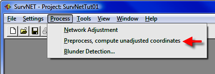
The Preprocess, compute unadjusted coordinates option allows the computation of unadjusted coordinates. If there are redundant measurements in the raw data, the first angle and distance found in the raw data is used to compute the coordinates. If a state plane grid system has been designated the measurements are reduced to grid prior to the computation of the unadjusted coordinates. If the point is located from two different points the initial computation of the point will be the value stored.

A variety of blunder detection tools are available that gives the user additional tools in analyzing his survey data, and detecting blunders. The standard least squares adjustment processing and its resulting report can often be used to determine blunders. No blunder detection method can be guaranteed to find all blunders. So much depends on the nature of the network geometry, the nature of the measurements, and the intuition of the analyst. Generally, the more redundancy there is in a network the easier it is to detect blunders.
There are three different methods that can be used to track down blunders in a network or traverse.
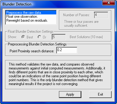
The Preprocess the raw data option validates the raw data. It displays angle and distance spreads as well as checks the validity of the raw data. Traverse closures are computed if specified. It also performs a K-Matrix analysis. The K-Matrix analysis compares the unadjusted, averaged measurements with the computed preliminary measurements (measurements calculated from the preliminary computed coordinates). This method will catch blunders such as using the same point number twice for two different points. The report will be sent to the .ERR file. The .ERR file will contain the tolerance checks, closures and the K-Matrix analysis. Following is an example of the report created using the Preprocess the raw data option. Notice that the first section of the report shows the angle and distance spreads from the multiple angle and distance measurements. The second part of the report shows the K-Matrix analyses.
Additionally there is a Point Proximity Report section that reports pairs of different points that are in close proximity to each other which may indicate where the same point was collected multiple times using different point numbers.
The Preprocess the raw data option is one of the simplest and effective tools in finding blunders. Time spent learning how this function works will be well spent. If the project is not converging due to an unknown blunder in the raw data this tool is one of the most effective tools in finding the blunder. Many blunders are due to point numbering errors during data collections, and the K-Matrix analysis and Point Proximity search are great tools for finding this type blunders.
=====================================
LEAST SQUARES ADJUSTMENT ERROR REPORT
=====================================


Tue Mar 21 16:04:32 2006

Input Raw Files:
    C:\data\lsdata\cgstar\CGSTAR.CGR
Output File: C:\data\lsdata\cgstar\cgstar.RPT
Checking raw data syntax and angle & distance spreads.


Warning: Missing Vert. Angle. Assumption made as to whether it is direct or reverse.
  1                                   5.00  180.00050                              4

Warning: Missing Vert. Angle. Assumption made as to whether it is direct or reverse.
  1                                   5.00  180.00070                              5

Warning: Missing Vert. Angle. Assumption made as to whether it is direct or reverse.
  1                                   5.00  180.00100                             10

Warning: Missing Vert. Angle. Assumption made as to whether it is direct or reverse.
  1                                   5.00  180.00020                             11

Warning: Missing Vert. Angle. Assumption made as to whether it is direct or reverse.
  1                                   5.00  325.54320                              2     H&T

Warning: Missing Vert. Angle. Assumption made as to whether it is direct or reverse.
  1                                   5.01  145.54300                              2     H&T

Warning: Missing Vert. Angle. Assumption made as to whether it is direct or reverse.
  1                                   5.01  180.00020                             12

Horizontal Angle spread exceeds tolerance:
  IP: 1,  BS: 5,  FS: 2
  Low: 109-19'10.0" ,  High: 109-19'17.0" ,  Diff: 000-00'07.0"


Horizontal Angle spread exceeds tolerance:
  IP: 2,  BS: 1,  FS: 6
  Low: 190-32'02.0" ,  High: 190-32'10.0" ,  Diff: 000-00'08.0"


Horizontal Angle spread exceeds tolerance:
  IP: 2,  BS: 1,  FS: 3
  Low: 096-03'48.0" ,  High: 096-03'56.0" ,  Diff: 000-00'08.0"


Horizontal Angle spread exceeds tolerance:
  IP: 3,  BS: 2,  FS: 4
  Low: 124-03'50.0" ,  High: 124-03'56.0" ,  Diff: 000-00'06.0"


Horizontal Angle spread exceeds tolerance:
  IP: 5,  BS: 4,  FS: 10
  Low: 039-26'35.0" ,  High: 039-26'45.0" ,  Diff: 000-00'10.0"


Horizontal Angle spread exceeds tolerance:
  IP: 10,  BS: 5,  FS: 11
  Low: 241-56'23.0" ,  High: 241-56'35.0" ,  Diff: 000-00'12.0"


Horizontal Angle spread exceeds tolerance:
  IP: 11,  BS: 10,  FS: 12
  Low: 114-56'20.0" ,  High: 114-56'34.0" ,  Diff: 000-00'14.0"


Horizontal Angle spread exceeds tolerance:
  IP: 12,  BS: 11,  FS: 3
  Low: 140-39'18.0" ,  High: 140-39'31.0" ,  Diff: 000-00'13.0"


Horizontal Angle spread exceeds tolerance:
  IP: 5,  BS: 4,  FS: 1
  Low: 117-30'35.0" ,  High: 117-30'50.0" ,  Diff: 000-00'15.0"


Horizontal Distance from 2 to 3 exceeds tolerance:
  Low: 324.15,  High: 324.20,  Diff: 0.04


Vertical Distance from 2 to 3 exceeds tolerance:
  Low: 6.62,  High: 8.36,  Diff: 1.74


Vertical Distance from 3 to 4 exceeds tolerance:
  Low: 11.46,  High: 11.51,  Diff: 0.05


Horizontal Distance from 12 to 3 exceeds tolerance:
  Low: 144.64,  High: 144.66,  Diff: 0.02
K-Matrix Analysis.


Distance: From pt.: 4  To pt.: 5
   Measured distance:    309.61  Initial computed distance:    309.65
   Difference:     -0.04


Distance: From pt.: 12  To pt.: 3
   Measured distance:    144.63  Initial computed distance:    144.66
   Difference:     -0.03


Distance: From pt.: 5  To pt.: 6
   Measured distance:    348.51  Initial computed distance:    523.29
   Difference:   -174.79


Angle: IP: 4  BS: 3  FS: 5
   Measured angle:          093-02'11.5"
   Initial computed angle:  093-01'45.1"
   Difference:  000-00'26.4"


Angle: IP: 12  BS: 11  FS: 3
   Measured angle:          140-39'24.5"
   Initial computed angle:  140-40'32.6"
   Difference: -000-01'08.1"


Angle: IP: 5  BS: 4  FS: 1
   Measured angle:          117-30'42.5"
   Initial computed angle:  117-31'16.4"
   Difference: -000-00'33.9"


Angle: IP: 5  BS: 4  FS: 6
   Measured angle:          145-30'34.0"
   Initial computed angle:  079-39'46.4"
   Difference:  065-50'47.6"


Point Proximity Report:
  Points  3  and 30 are within      0.05 of each other.
The problem with the above project was that point 6 was accidentally used twice for two separate side shots. Because of the point numbering problem the project would not converge using the regular least squares processing. The Preprocess the raw data option was then used. Notice in the K-matrix section the distance from 5 to 6 shows a difference of 174.79' and the angle 4-5-6 shows a difference of 065-50'47.6". Then notice that the other listed differences are in the range of .02' for the distances and less than a minute for the angles. This report is clearly pointing out a problem to point 6.
Note the point
proximity report section. During data collection point number 30 was used
as the point number when the point was previously collected as point 3.
In the first section of the report notice that there are several warnings
concerning whether a horizontal angle reading was collected in direct or reverse
reading. The preprocessing software uses the vertical angle reading to
determine the angle face of the horizontal angle reading. If the vertical
angle is missing the program makes its best guess as to whether the angle was
collected in direct or reverse face. Since all horizontal angle spreads in
the report are reasonable, the preprocessing software must have made the correct
determination.
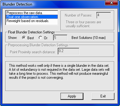
This option is
useful in finding a single blunder, either an angle or distance, within a
network or traverse. If there is more than a single blunder in the network
then it is less likely that this method will be able to isolate the blunders.
If the standard least squares processing results in a network that will not
converge then this blunder detection method might not work. Use the
Preprocess the raw data blunder detection method if the solution is not
converging. Also this method will only work on small and moderately sized
networks. This method performs a least squares adjustment once for every
non-trivial measurement in the network. So for large networks this method
may take so long to process that it is not feasible to use this method.
With this method an adjustment is computed for each non-trivial individual angle
and distance measurement. Consecutively, a single angle or distance
is allowed to float during each adjustment. The selected floated angle or
distance does not "constrain" the adjustment in any way. If there is a
single bad angle or distance, one of the adjustment possibilities will place
most of the error in the "float" measurement, and the other measurements should
have small residuals. The potentially bad angle or distance is flagged
with a double asterisk (**).
Since an adjustment is computed for each measurement this method my take a long
time when analyzing large data files.
The adjustments with the lowest reference variances are selected as the most
likely adjustments that have isolated the blunder. You have the choice to
view the best adjustment, or the top adjustments with a maximum of ten. In
the above example we asked to see the top five choices for potential blunders.
The results are shown in the .ERR file. Following is a section of
the report generated where an angular blunder was introduced into a small
traverse. Notice the '**'
characters beside the angle measurements. In this report the two most
likely adjustments were displayed. The blunder was introduced to angle
101-2-3. Angle 101-2-3 was chosen as the 2nd most likely source of the
blunder, showing that these blunder detection methods though not perfect, can be
a useful tool in the analysis of survey measurements. Notice how much
higher the standard residuals are on the suspected blunders than the standard
residuals of the other measurements.
Adjusted Observations
=====================


Adjusted Distances

From Sta.  To Sta.      Distance      Residual     StdRes.   StdDev

101           2           68.780      -0.006        0.608     0.008
2             3           22.592      -0.006        0.573     0.008
3             4           47.694      -0.002        0.213     0.008
4             5           44.954      -0.001        0.069     0.008
5             6           62.604       0.005        0.472     0.009
6             7           35.512       0.006        0.539     0.008
7             101         61.704       0.003        0.314     0.009

           Root Mean Square (RMS)      0.005


Adjusted Angles

BS Sta. Occ. Sta.  FS Sta.    Angle       Residual     StdRes    StdDev(Sec.)
7          101      2        048-05'06"       -5          0          21
101        2        3        172-14'33"       -2          0          27
2          3        4        129-27'44"     -222   *      7          56   **
3          4        5        166-09'59"       11          0          25
4          5        6        043-12'26"       22          1          21
5          6        7        192-11'52"       12          0          25
6          7        101      148-38'19"        8          0          25

                  Root Mean Square (RMS)      85


Adjusted Azimuths

Occ. Sta.  FS Sta.      Bearing           Residual     StdRes    StdDev(Sec.)

101         7          N 00-00'00"E            0          0           4

               Root Mean Square (RMS)          0


Statistics
==========

Solution converged in 2 iterations
Degrees of freedom:3
Reference variance:0.78
Standard error unit Weight: +/-0.88
Passed the Chi-Square test at the 95.00 significance level
0.216 <= 2.347 <= 9.348


Adjusted Observations
=====================


Adjusted Distances

From Sta.  To Sta.      Distance      Residual     StdRes.   StdDev
101           2           68.781      -0.005       0.473      0.009
2             3           22.592      -0.005       0.512      0.009
3             4           47.690      -0.006       0.586      0.009
4             5           44.950      -0.005       0.523      0.009
5             6           62.605       0.006       0.607      0.009
6             7           35.512       0.006       0.560      0.009
7             101         61.708       0.006       0.614      0.009

           Root Mean Square (RMS)      0.006


Adjusted Angles

BS Sta.  Occ. Sta.   FS Sta.    Angle        Residual    StdRes  StdDev(Sec.)

7         101         2        048-05'22"       11           0        24
101       2           3        172-11'03"     -213    *      7        58   **
2         3           4        129-31'23"       -3           0        29
3         4           5        166-09'48"        1           0        26
4         5           6        043-12'11"        6           0        21
5         6           7        192-11'50"       10           0        27
6         7           101      148-38'24"       13           0        27

                   Root Mean Square (RMS)       81


Adjusted Azimuths

Occ. Sta.  FS Sta.      Bearing           Residual       StdRes  StdDev(Sec.)

101         7          N-00-00'00"E            -0            0         5

                Root Mean Square (RMS)          0


Statistics
==========


Solution converged in 2 iterations
Degrees of freedom:3
Reference variance:0.89
Standard error unit Weight: +/-0.94
Passed the Chi-Square test at the 95.00 significance level
0.216 <= 2.675 <= 9.348
The blunder is most likely in the measurement containing the largest residual and standard residual. The observation marked with ** is the observation that floated. It is also most likely the measurement containing the blunder.
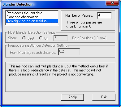
This method is capable of detecting multiple blunders but one is more likely to find the blunders if there is a high degree of redundancy (network of interconnected traverses). The higher the degree of freedom the more likely this method will find the blunders. This method will not work if the standard least squares processing will not converge. Use the Preprocess the raw data blunder detection method if the network is not converging.
First, select the number of adjustments or passes you wish to make. Each time an adjustment is completed, the measurements will be re-weighted based on the residuals and standard errors. Hopefully after three or four passes the blunders will become obvious. The results are shown in the .ERR file, look for the measurements with the highest standard residuals. These measurements are more likely to contain blunders.
The theory behind this method is that after processing, the measurements with blunders are more likely to have higher residuals and computed standard errors. So, in the next pass the measurements are re-weighted based on the computed residuals, with less weight being assigned to the measurements with high residuals. After several passes it is likely that the measurements with the blunders have been reweighed such that they have little effect on the network.
As a rule of thumb three or four passes are usually sufficient. Following is a section of the report showing the results of the Reweight by residuals & std. err. This report was generated using the same data used in the earlier example. Notice that it has flagged the same two angle measurements.
The Reweight by residuals & std. err. method performs a new adjustment for each pass; so this method will take longer than the standard least squares adjustment, but does not take near as long to complete processing as the Float one Observation method for larger networks.
=====================
Adjusted Observations
=====================


Adjusted Distances

From Sta.  To Sta.        Distance    Residual     StdRes.   StdDev

101           2             68.778      -0.009       0.827    0.014
2             3             22.588      -0.010       0.942    0.015
3             4             47.694      -0.002       0.208    0.009
4             5             44.954      -0.001       0.077    0.006
5             6             62.608       0.010       0.919    0.016
6             7             35.517       0.011       1.040    0.016
7             101           61.705       0.004       0.398    0.011

             Root Mean Square (RMS)      0.008


Adjusted Angles

BS Sta.  Occ. Sta.   FS Sta.       Angle        Residual    StdRes   StdDev(Sec.)

7         101         2          048-05'07"        -4          0         21
101       2           3          172-13'19"       -77     *    2         65
2         3           4          129-29'56"       -91     *    3         64
3         4           5          166-09'44"        -3          0         24
4         5           6          043-12'05"         0          0          9
5         6           7          192-11'40"        -0          0         19
6         7           101        148-38'10"        -1          0         20

                   Root Mean Square (RMS)          45


Adjusted Azimuths

Occ. Sta.  FS Sta.        Bearing           Residual       StdRes    StdDev(Sec.)
101          7          N 00-00'00"E            0             0            2

                Root Mean Square (RMS)          0


Statistics
==========

Solution converged in 1 iterations
Degrees of freedom:3
Reference variance:1.77
Standard error unit Weight: +/-1.33
Passed the Chi-Square test at the 95.00 significance level
0.216 <= 5.322 <= 9.348
The blunder is most likely in the measurement containing the largest residual and standard residual.
SurvNET provides a window that graphically displays the survey network. Additionally the user is able to display error ellipses, and GPS vectors. The user has much control over how the network is displayed. The graphic tool is a useful tool in debugging networks since the raw data can be displayed prior to adjustment. If there are problems with the raw data the graphics often reflect the problem. The actual graphics cannot be output or saved. The graphics can be shown independent of whether the project has been processed.
The following illustration shows a view of the graphic window, which can be accessed using the eye icon on the main tool bar. A project must be opened before the graphic window can be displayed. The graphics window will only display error ellipses after the project has been processed.
The tool bar in the graphics window contains buttons that allow the user to pan, zoom in, zoom out, zoom extents, and zoom to a window. Additionally there is a button that allows the user to navigate to points in the .CGR raw data editor. Also, there are buttons that will refresh the graphic, and change the graphic settings.
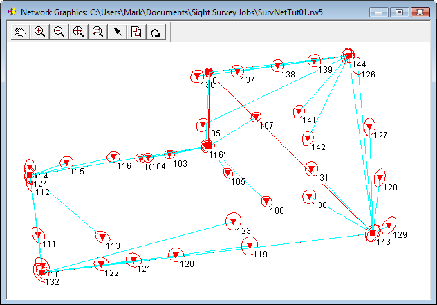
|
|
Pan: Use this button to pan the graphics. |
|
|
Zoom In: Use this button to zoom in on the graphics. |
|
|
Zoom Out: Use this button to zoom out on the graphics. |
|
|
Zoom Extents: Use this button to zoom to the extents of the graphics. |
|
|
Zoom to Wwindow: Use this button to zoom to the extents of a user picked window. |
|
|
Pick Point: This button allows the user to navigate within the .CGR raw editor from the graphics window. Currently this button serves no purpose when working with .RW5 data. |
|
|
Settings: This buttons is used to change the graphic display settings. |
|
|
Refresh: This button will refresh the graphic view. Graphics are generated from the saved raw data file. If you make changes to the raw file in the raw editor you must save the file before the changes will be reflected in the refreshed graphic screen. |
Following is a description of the options in the graphics setting dialog box, which is accessed using the Settings tool bar button.
These settings determine how the different type control points are displayed in the graphics window. Different graphic settings can be applied to standard control points, fixed control points and floating control points. The symbol node display can be controlled as to symbol type, symbol color, symbol size. The control point name can be displayed and its size set from this setting dialog box.
The graphic pick radius defines a search radius. This radius is used when navigating the .CGR editor using the graphic window. You can pick a point graphically and the cursor in the editor will go to the next field containing that point number. The radius is defined in terms of the distance units of the raw data file.
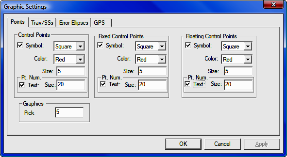
These settings determine how the network line work will be displayed for total station raw data. There are settings for traverse data, side shot data, and azimuth control. The program considers any point that has only a single angle and distance to it a side shot. The user can control the color of the traverse lines. The symbol node display can be controlled as to symbol type, symbol color, symbol size. The point name can be displayed and its size set from this setting dialog box.
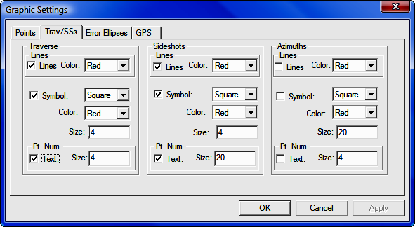
These settings determine how the error ellipses will be displayed in the graphic window. Error ellipses will only be displayed if there is a successful least squares adjustment. The display of the error ellipses is relative, and the program automatically determines a default relative error ellipse size. The user can modify the visual size of the error ellipses using the track bar in the following dialog box. The user can also control the color of the error ellipse from the following dialog box.
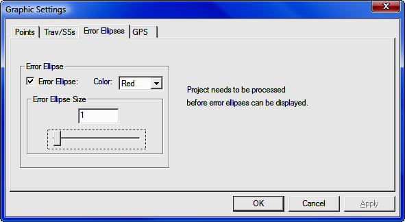
The settings in the following dialog box determine how GPS vectors will be displayed in the graphic window. The user can control the color of the GPS vector lines. The symbol node display can be controlled as to symbol type, symbol color, symbol size. The GPS point names can be displayed and their size set from this setting dialog box.
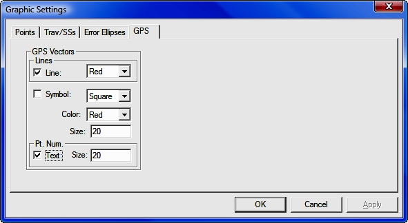
Some statutes and jurisdictions still require the computation of traditional traverse closures. SurvNET gives the surveyor the ability to compute the closures of multiple traverses within a project as part of the preprocessing of the project raw data. Closures for single or multiple traverses can be computed for a single project. Additionally, GPS closures can be computed for GPS loops. To compute closures you must first create a Closure file (.CLS). Closure files define the type of traverse loops that are to be computed and the point numbers that make up the traverse.
There are two options in the FILE menu that are used to create and edit the closure files (.cls):
Open Traverse Closure File
New Traverse Closure File
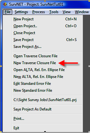
After choosing the New Traverse Closure File you will be prompted for a new file name. After choosing a file name the following dialog box is displayed.
First enter the point sequence which defines the traverse in the Ordered Traverse Point List grid field. Set the check boxes to set whether vertical closure and angle closures are to be computed, then choose what type traverse is being entered.
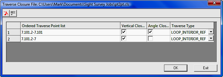
Enter the points that define
the traverse. Points can be entered in the form: 1,23,30-35,45,23,1
A comma separates the point numbers. You can select a range (30-35) when the
points are sequential. You must start with the first backsight point
number and end with the last foresight point number. For example, if you
have a simple loop traverse with angle closure using points 1, 2, 3 and 4, it
will be entered as: 4,1,2,3,4,1 where 1 is the first occupied
point and 4 is the initial backsight.
You can set the Angle Closure as ON or OFF. If the
angle closure is ON, you will be shown the total angular error and error
per angle point. If the final closing angle was not collected you can set
Angle Closure to OFF and only the linear closure will be computed.
You can set the Vertical Closure as ON or OFF. If the
vertical closure is ON, you will be shown the total vertical distance
closure.
In order to calculate the traverse closure, you must select the TRAVERSE TYPE.
It can be:
Pt. to Pt. Trav. - A point to point traverse is a traverse that starts at
a set of known coordinates and ends at another known coordinate. This
option assumes you start from two control points and tie into two control points
if an angle closure is desired and one control point if only a linear closure is
desired. The first backsight distance and last foresight distance if angle
closure is ON are not used in computing the linear closure.
Following is an example of a pt. to pt. traverse with angle closure.
100,101,2-5
In the above pt. to pt. list Pt 100 is the starting backsight point, Pt. 101 is the starting instrument point. Pt. 4 is the ending instrument point and the foresight to the angle closure point is point 5. If a closing angle was not collected the list would look as follows: 100,101,2-4
Loop Trav., Int. Az. Ref. - A closed loop traverse that begins by back sighting the last interior point on the traverse. Following is an example.
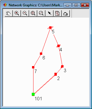
7,101,2-7,101
In the above example closed loop with angle balance list, point 7 is the backsight point and point 101 is the first occupied point. If the closing angle 6-7-101 was not collected the list would be entered as follows: 7,101,2-7
Loop Trav., Ext. Az. Ref. - A closed loop traverse that begins by back sighting an exterior point (point not on the traverse).
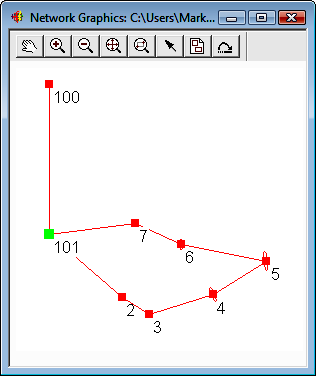
100,101,2-7,101,100
In the above example loop with exterior reference and angle balance list, point 100 is the backsight point and point 101 is the first occupied point. If the closing angle 7-101-101 was not collected the list would be entered as follows: 100,101,2-7,101
GPS Loop Closure: - GPS loop closures can be computed using this option.

A,E,F,A
In the above example GPS loop, closure will be computed from the GPS loop going from A-E-F-A.
After the closure file (.cls) has been created the preprocessing project settings need to be updated to include the closure file in the project. Following is a view of the settings screen that defines a closure file to be used in preprocessing. Notice that the check box Compute Traverse Closure is checked and a closure file has been entered in the edit box field. Notice that the [Edit/Create] button can be used to edit an existing closure file or create a new closure file.
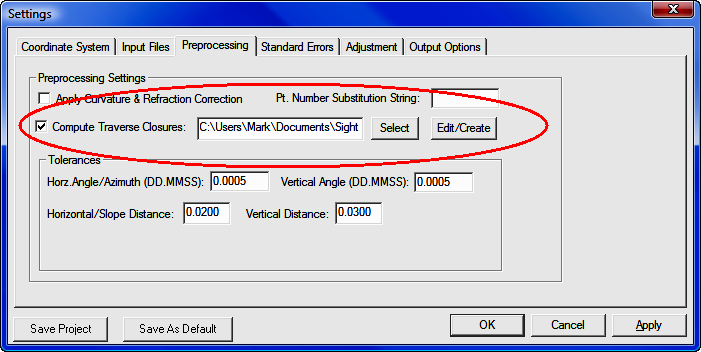
When the data is processed, the closure reports will appear in the RPT and ERR files. Following is an example of a closed loop traverse report:
Traverse Closures
=================

Traverse points:
7,101,2-7,101

Loop Traverse; Interior direction reference;
Compute angle closure.
Do not compute vertical closure.


Total angular error:  000-04'16"
Angular error per point:  000-00'37"


Correct Ending Coordinates, North: 249369.069 East: 642232.387
Ending Coordinates, North: 249369.156 East: 642232.360
Error, N: 0.087 E: -0.026 Total: 0.091 Brg:    S 16-46'01"E
Distance Traversed:   344.651 Closure:  3776.794
Following is an example of a GPS loop closure report.
Traverse Closures
=================


GPS Loop Points:
A,E,F,A


GPS Loop Closure;
Misclosure, X:  -0.0323   Y:  -0.0162   Z:  -0.0105
Closure error:    0.0376   Perimeter: 20229.3858
Precision: 1:537594


GPS Loop Points:
C,F,D,B,C


GPS Loop Closure;
Misclosure, X:  -0.0121   Y:  -0.0101   Z:   0.0002
Closure error:    0.0158   Perimeter: 41332.9807
Precision: 1:2622216


GPS Loop Points:
F,D,B,F


GPS Loop Closure;
Misclosure, X:  -0.0022   Y:  -0.0044   Z:   0.0097
Closure error:    0.0109   Perimeter: 30814.5047
Precision: 1:2833226
Following is a view of the closure file that created the above GPS closure report. The Vert. Closure and Angle Closure toggles serve no purpose with GPS loop closures.
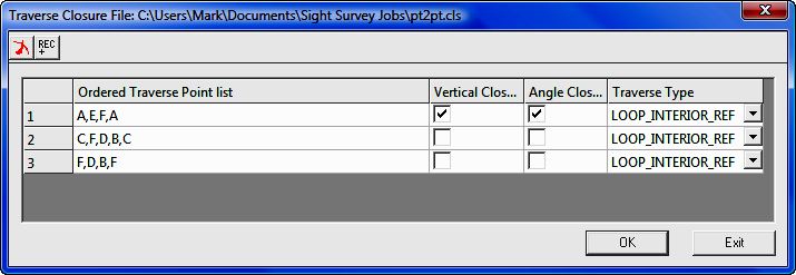
SurvNET provides the ability to generate reports that give the surveyor the information needed to determine if his survey is within ALTA positional tolerances. It is required that the user define which points are to be included in the ALTA testing. The points to be included for ALTA testing are defined in an .Alt file.
There are two options in the FILE menu that are used to create and edit the
ALTA files (.alt):
Open ALTA, Rel. Err. Ellipse File
New ALTA, Rel. Err. Ellipse File
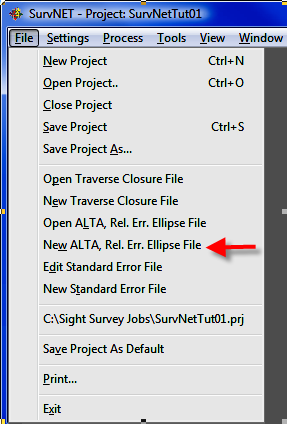
After choosing the ALTA file to be created or edited the following dialog box is displayed.
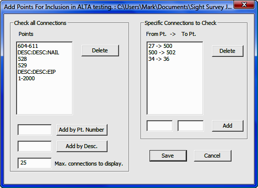
The above dialog box allows
the user to define the points to be included in the ALTA report processing.
There are two sections in the .RPT file created through the ALTA reporting.
The following report shows the sections of the ALTA report generated by the data
in the dialog box. The first section of the report displays only the
relative error ellipses between points. The point sequences used in this
section come from the list on the right hand side of the above dialog box.
The second section of the report performs an ALTA tolerance test and displays
only those connections that fall outside of the ALTA tolerances (as set in the
ADJUSTMENT tab of the SETTINGS dialog box). The program
first checks the specific point sequences defined by the list on the right side
of the dialog box. The program then checks all the connections between all
the points listed on the left hand side of the dialog box.
There can be many connections to check if the point list on the left hand side
of the dialog box has a lot of points. The user can limit the number of
sequences to be displayed that fail the ALTA test by entering a number in the
Max. Connections to display field.
Notice that you can enter points based on descriptions in the left hand list
box. If you wished to check connections between all points with TP, EIP,
MON descriptions, enter the descriptions in the edit field and press the [Add]
button. If TP, EIP, and MON represented traverse points, existing iron
pipes and monuments then ALTA testing would be performed on those point types.
After you have created the .ALT point file you need to set a few project settings. These settings define the ALTA tolerances, specify the .ALT file to be used, and define the type of reporting to be generated. The Adjustment tab sheet within the Project Settings, has a relative error ellipse section where the ALTA report settings are located.
All the ALTA reporting settings reside within the Relative Error Ellipse box. If there are any side shots that need to be included in the ALTA testing, the Enable side shots for relative error ellipses check box must be checked.
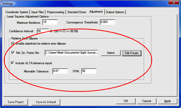
The Rel. Err. Points File check box must be checked, and an .ALT file must be chosen to get an ALTA report. The .ALT file defines which points will be included in the ALTA reporting. See the previous discussion on the creation of the .ALT file if you are unsure of how to create an .ALT file.
Check the Include ALTA tolerance report check box to create the ALTA tolerance checking report section. I f an .ALT file has been chosen then the relative error section of the report will always be generated.
Next make sure the appropriate tolerance and PPM has been defined. The ALTA standards define their positional standard as .07 plus 50 PPM. Additionally, the ALTA standards require that the computations be performed to a 95% confidence. The confidence interval is set in the Confidence Interval edit field.
After the project has been processed the ALTA/Relative Error portion of the report is displayed in the report window under the ALTA/Relative Err. tab.
The following is a sample ALTA report:
Relative Error and ALTA Tolerances
==================================


Alta Tolerance Report ,Specific Connections, 95% Confidence Interval

                            Actual     Allowable     Ratio
Sta.   Sta.      Dist.    Semi Major  Semi Major  Actual/Allow.  Semi Minor    Max. Err. Az.
27     500     204.5030     0.0793      0.0802      0.9890         0.0588     S 85-06'32.2"E
500    502      66.8572     0.1132      0.0733      1.5432         0.0842     S 86-05'06.7"E
34      36     237.9748     0.0731      0.0819      0.8920         0.0731     N 00-00'00.0"E


Alta Tolerance Report ,All Connections, 95% Confidence Interval

                            Actual     Allowable     Ratio
Sta.   Sta.      Dist.    Semi Major  Semi Major  Actual/Allow.  Semi Minor    Max. Err. Az.
506    556     806.5402     1.0818      0.1103      9.8054         0.2586     S 86-37'40.4"E
507    556     827.2364     1.0832      0.1114      9.7268         0.2446     S 86-37'05.9"E
505    556     818.7994     1.0779      0.1109      9.7158         0.2386     S 86-48'24.5"E
508    556     854.9436     1.0836      0.1127      9.6108         0.2477     S 86-38'39.4"E
509    556     880.6338     1.0848      0.1140      9.5129         0.2489     S 86-45'39.4"E
521    556     798.2729     1.0387      0.1099      9.4500         0.2318     S 87-22'50.2"E
512    556     793.0518     1.0334      0.1097      9.4245         0.2127     S 87-21'38.9"E
517    556     907.2084     1.0856      0.1154      9.4106         0.2379     S 87-07'38.4"E
510    556     918.6572     1.0861      0.1159      9.3682         0.2525     S 86-52'46.5"E
516    556     935.1194     1.0885      0.1168      9.3228         0.2426     S 87-22'21.7"E
511    556     941.3134     1.0830      0.1171      9.2516         0.2283     S 87-33'40.2"E
518    556     962.0899     1.0893      0.1181      9.2231         0.2345     S 87-36'45.6"E
550    556     656.1441     0.9453      0.1028      9.1946         0.1952     S 87-09'41.3"E
515    556     978.6797     1.0882      0.1189      9.1495         0.2484     S 87-34'16.6"E
513    556     981.5606     1.0893      0.1191      9.1477         0.2452     S 87-42'02.1"E
514    556     985.2691     1.0895      0.1193      9.1349         0.2454     S 87-41'57.3"E
519    556     993.3973     1.0904      0.1197      9.1116         0.2388     S 87-32'58.7"E
504    556    1004.0126     1.0838      0.1202      9.0163         0.2643     S 86-11'23.8"E
520    556    1132.1493     1.0918      0.1266      8.6234         0.2423     S 87-17'23.7"E
524    556    1152.1979     1.0948      0.1276      8.5796         0.2993     S 86-39'15.0"E
551    556     530.9691     0.8252      0.0965      8.5471         0.1766     S 87-17'08.2"E
506    555     695.5978     0.8953      0.1048      8.5450         0.2389     S 86-24'27.4"E
556    800    1161.6986     1.0945      0.1281      8.5449         0.2766     S 86-03'20.2"E
503    556    1172.1735     1.0945      0.1286      8.5101         0.2767     S 86-03'36.5"E
522    556    1164.2729     1.0911      0.1282      8.5100         0.2546     S 86-47'21.4"E
If the Ratio Actual/Allowable is 1.0 or less, the positional tolerance of the two points have passed the ALTA standards. The first part of the report labeled Specific Connections will show all selected connections whether they passed or failed. The second part of the report, labeled All Connections will only show the connections that "failed" (we chose to see the worst 25).
GPS vector networks can be adjusted with the current version of SurvNET. This section will describe the processing of a simple GPS network. Following is a graphic view of the GPS network that is to be adjusted. Points A and B are control points. The red lines represent measured GPS vectors. Most GPS vendor's software can output GPS vectors to a file as part of the post processing of GPS data.
When processing GPS vectors certain project settings are important. In the following settings dialog box notice that the 3D-model has been chosen, and SPC 1983 with an appropriate zone has been chosen. The 3-D model and a geodetic coordinate are required when processing GPS vectors. Though it is not require for GPS processing it is in most cases appropriate to chose to do geoid modeling, especially if the project covers a large extents. The following settings dialog box shows the raw files used in processing GPS files. A GPS vector file must be chosen.
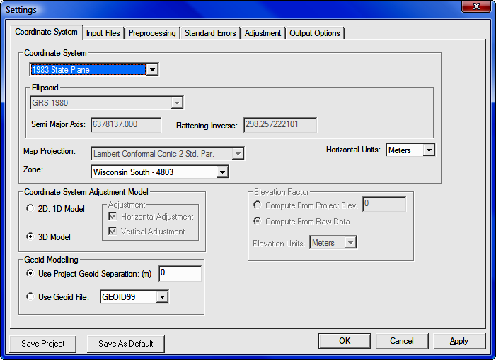
GPS vector files from various GPS vendors are currently supported. Following are the formats currently supported.
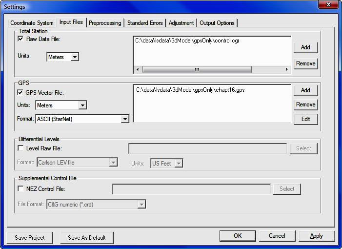
Coordinate control for the network can be in one of several files. The control can be located in the GPS vector file itself. More typically, the control points can be regular coordinate records in the .RW5 or the .CGR file. The also can be entered as Supplemental Control in one of the available formats. When the control coordinates are in the raw data file or supplemental coordinate file, the coordinates are expected to be grid coordinates. If the control coordinates are found in the GPS vector file, they are assumed to be Earth centered XYZ.
Very often the point numbering convention used in the GPS data collection is different than the point number convention used when collecting total station data. If the point numbers in the GPS file differ from the total station point number it is easy to first convert the native GPS format file to a ASCII .GPS using the Tools/Convert GPS file to ASCII menu option. The .GPS ASCII files can easily be edited to ensure point numbers are consistent between GPS and total station data.
It is not unusual to have different distance units for GPS, total station data, and control data. Often the GPS vector data is in metric units but the total station raw file is in US Feet, so the distance units must be specified for the different raw data types.
In the Preprocessing Settings dialog box the only important setting is the Compute Traverse Closures options. If GPS loop closures need to be computed, the loop point numbers need to be entered into a closure file. See the section on traverse closures to see how to create closure files.
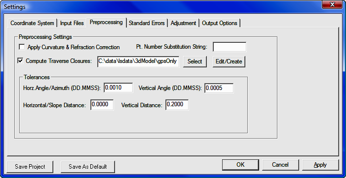
There are two GPS Standard Errors fields in the Standard Errors dialog box. The GPS vector XYZ standard errors and covariances do not need to be defined as project settings since they are typically found in the GPS vector data files. The Instrument centering standard error is the estimated error in centering the GPS unit over the survey point. The Vector Std. Err. Factor can be used to globally increase the variance/covariances found in the GPS files without having to edit the GPS file itself.
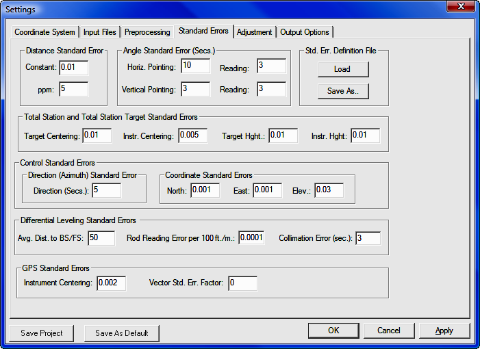
The following section shows the report generated by the least squares adjustment of the GPS network. Explanations of the report are included following each report section.
===============================
LEAST SQUARES ADJUSTMENT REPORT
===============================


Mon May 08 13:03:02 2006

3D Geodetic Model.

Input Raw Files:
    C:\data\lsdata\3dModel\gpsOnly\control.cgr
GPS File:  C:\data\lsdata\3dModel\gpsOnly\chapt16.gps
Output File: C:\data\lsdata\3dModel\gpsOnly\gpsOnlyl.RPT
Traverse File: C:\data\lsdata\3dModel\gpsOnly\gpsLoops.cls

Curvature, refraction correction: OFF

Maximum iterations: 10 , Convergence Limit: 0.002000
1983 State Plane Coordinates, zone:4803 Wisconsin South
Horizontal Units: Meters
Confidence Interval: 95.00
Project Geoid Height:    0.0000

Default Standard Errors:
Distance: Constant 0.010 ,PPM: 5.000
Horiz. Angle: Pointing 10.0" ,Reading: 3.0"
Vert. Angle: Pointing 3.0" ,Reading: 3.0"
Total Station: Centering 0.005 ,Height: 0.010
Target: Centering 0.010 ,Height: 0.010
Azimuth: 5"

Coordinate Control: N:0.001, E:0.001, Z:0.030,
GPS: Centering:0.000, Vector Err. Factor:1.0
The following section shows the unadjusted measurements that make up the network. The control coordinates are displayed first followed by the GPS vectors. The control coordinates are displayed as latitude/longitude, SPC Grid XYZ, and geocentric XYZ. If geoid modeling is set both ellipsoid and orthometric elevations are displayed, ellipsoid elevation in the latitude/longitude section and orthometric elevation in the SPC section. The GPS vector section shows the unadjusted delta XYZ, variances and covariances of the vectors.
Unadjusted Observations
=======================


Control Coordinates:    0 Observed Points,   2 Fixed Points,   0 Approx. Points


 Sta.    Latitude         Longitude      Z (Ellip.)  StErr N:  StErr E:   StErr
Z:


 A   43-15'46.28901"N   89-59'42.16399"W   1382.62      FIXED     FIXED     FIXED
 B   43-23'46.36261"N   89-54'00.75701"W   1235.46      FIXED     FIXED     FIXED


Grid XYZ
 Sta.        N:            E:         Z (Geoid):   StErr N:   StErr E:   StErr
Z:


 A       140291.2060   600402.2380       1382.62      FIXED      FIXED      FIXED
 B       155110.5390   608083.9250       1235.46      FIXED      FIXED      FIXED
Geocentric XYZ
Sta. X: Y:
Z: StErr X: StErr Y: StErr
Z:
A 402.3510 -4652995.3008 4349760.78 FIXED FIXED
FIXED
B 8086.0316 -4642712.8473 4360439.08 FIXED FIXED
FIXED
GPS Vectors: 13 Observations
From Sta. Delta X Variance Delta X Covariance XY
To Sta. Delta Y Variance Delta Y Covariance XZ
Delta Z Variance Delta Z Covariance YZ
A 11644.223 0.001969 -1.916E-005
C 3601.217 0.001875 1.904E-005
3399.255 0.001965 -1.904E-005
A -5321.716 0.0004316 -4.2E-006
E 3634.075 0.0003838 4.32E-006
3173.665 0.000401 -4.2E-006
B 3960.544 0.000461 -4.46E-006
C -6681.247 0.0005092 4.14E-006
-7279.015 0.0004504 -4.46E-006
B -11167.608 0.00054 -5.5E-006
D -394.520 0.0005442 5.7E-006
-907.959 0.000534 -5.44E-006
D 15128.165 0.0002922 -2.86E-006
C -6286.705 0.0003228 2.68E-006
-6371.058 0.0002616 -2.88E-006
D -1837.746 0.0002462 -2.38E-006
E -6253.853 0.0002554 2.44E-006
-6596.670 0.0002566 -2.42E-006
F -1116.452 0.0001495 -1.58E-006
A -4596.161 0.0001319 1.76E-006
-4355.906 0.0001523 -1.62E-006
F 10527.785 0.0005134 -4.5E-006
C -994.938 0.0004326 4.8E-006
-956.625 0.0004794 -4.54E-006
F -6438.136 0.0001889 -1.84E-006
E -962.069 0.0001992 2.08E-006
-1182.230 0.0001765 -1.78E-006
F -4600.379 0.0001866 -1.98E-006
D 5291.779 0.0001975 1.8E-006
5414.431 0.0002408 -1.98E-006
F 6567.231 0.0001329 -1.3E-006
B 5686.293 0.0001493 1.38E-006
6322.392 0.000121 -1.28E-006
B -6567.231 0.0001103 -1.26E-006
F -5686.303 0.0001495 1.22E-006
-6322.381 0.0001326 -1.26E-006
A 1116.458 0.0001324 -1.6E-006
F 4596.155 0.0001622 1.8E-006
4355.914 0.0001875 -1.64E-006
The
optional Traverse Closure section shows the GPS loop closures for the GPS loops
defined in the closure file (.CLS).
Traverse Closures
=================
GPS Loop Points:
A,E,F,A
GPS Loop Closure;
Misclosure, X: -0.0323 Y: -0.0162 Z: -0.0105
Closure error: 0.0376 Perimeter: 20229.3858
Precision: 1:537594
GPS Loop Points:
C,F,D,B,C
GPS Loop Closure;
Misclosure, X: -0.0121 Y: -0.0101 Z: 0.0002
Closure error: 0.0158 Perimeter: 41332.9807
Precision: 1:2622216
GPS Loop Points:
F,D,B,F
GPS Loop Closure;
Misclosure, X: -0.0022 Y: -0.0044 Z: 0.0097
Closure error: 0.0109 Perimeter: 30814.5047
Precision: 1:2833226
Following are the final adjusted coordinates. Included in the report are point grid factor, elev. factor and the combined factor. Following the adjusted coordinates are the error ellipses, followed by the adjusted measurements section.
Adjusted Geographic Coordinates
Adjusted Grid Coordinates, (Meters)

Sta.        N:            E:         Z (Geoid):  StErr N:   StErr E:  StErr Z:

C        145233.5553   612043.7117      1103.10    0.0062     0.0062    0.0060
E        145091.9380   595081.6888       914.98    0.0053     0.0053    0.0052
D        154179.9383   596919.0552       894.01    0.0051     0.0050    0.0052
F        146611.7860   601518.4564      1024.24    0.0029     0.0027    0.0028
Adjusted Geocentric Coordinates, (Metric)

Sta.       X:            Y:              Z:      StErr X:   StErr Y:  StErr Z:

C        12046.5807  -4649394.0824   4353160.06    0.0062     0.0062    0.0060
E        -4919.3403  -4649361.2195   4352934.45    0.0053     0.0053    0.0052
D        -3081.5836  -4643107.3693   4359531.12    0.0050     0.0051    0.0052
F         1518.8008  -4648399.1451   4354116.69    0.0027     0.0029    0.0028


Adjusted XYZ Coordinates Error Ellipses, 95% CI

Sta.               Semi Major      Semi Minor        Max. Error Az.       Elev.
                       Axis           Axis

C                    0.0161          0.0159          S 25-49'31.6"E      0.0157
E                    0.0138          0.0137          S 29-24'51.2"E      0.0136
D                    0.0133          0.0130          S 11-30'48.4"E      0.0135
F                    0.0074          0.0070          S 05-18'52.7"E      0.0073


Adjusted Observations
=====================


GPS Vectors:   13 Observations

From Sta.            Delta X    Residual     StdRes     StdDev
To   Sta.            Delta Y    Residual     StdRes     StdDev
                     Delta Z    Residual     StdRes     StdDev


A                  11644.2435    0.0203      0.4581     0.0062
C                   3601.2230    0.0065      0.1502     0.0062
                    3399.2795    0.0245      0.5521     0.0060


A                  -5321.7125    0.0039      0.1894     0.0053
E                   3634.1005    0.0251      1.2810     0.0053
                    3173.6781    0.0129      0.6429     0.0052


B                   3960.5330   -0.0112      0.5219     0.0062
C                  -6681.2418    0.0049      0.2181     0.0062
                   -7279.0098    0.0050      0.2378     0.0060


B                 -11167.6067    0.0009      0.0406     0.0050
D                   -394.5281   -0.0077      0.3288     0.0051
                    -907.9606   -0.0013      0.0568     0.0052


D                  15128.1644   -0.0003      0.0194     0.0063
C                  -6286.7131   -0.0077      0.4275     0.0064
                   -6371.0592   -0.0009      0.0573     0.0061


D                  -1837.7566   -0.0107      0.6844     0.0056
E                  -6253.8502    0.0032      0.2006     0.0057
                   -6596.6687    0.0010      0.0619     0.0057


F                  -1116.4498    0.0025      0.2079     0.0027
A                  -4596.1557    0.0053      0.4606     0.0029
                   -4355.9139   -0.0077      0.6259     0.0028


F                  10527.7799   -0.0053      0.2318     0.0061
C                   -994.9372    0.0005      0.0223     0.0061
                    -956.6272   -0.0026      0.1175     0.0060


F                  -6438.1411   -0.0047      0.3391     0.0050
E                   -962.0744   -0.0050      0.3507     0.0051
                   -1182.2367   -0.0062      0.4631     0.0050


F                  -4600.3844   -0.0057      0.4188     0.0047
D                   5291.7758   -0.0027      0.1889     0.0048
                    5414.4321    0.0010      0.0615     0.0050


F                   6567.2308   -0.0003      0.0220     0.0027
B                   5686.2978    0.0052      0.4292     0.0029
                    6322.3917   -0.0000      0.0037     0.0028


B                  -6567.2308    0.0003      0.0248     0.0027
F                  -5686.2978    0.0055      0.4474     0.0029
                   -6322.3917   -0.0110      0.9511     0.0028


A                   1116.4498   -0.0079      0.6903     0.0027
F                   4596.1557    0.0004      0.0321     0.0029
                    4355.9139   -0.0002      0.0128     0.0028
The final section displays a variety statistical measures, followed by side
shots if there are any. Side shots would be a point that has only a single
GPS vector going to or from the point.
Statistics
==========


Solution converged in 2 iterations
Degrees of freedom:27
Reference variance:0.26
Standard error unit Weight: +/-0.51
Failed the Chi-Square test at the 95.00 significance level
14.573 <= 6.927 <= 43.195
Processing a GPS vector network together with conventional total station data is similar to processing a GPS network by itself. The only difference in regards to project settings is that a raw data file containing the total station data needs to be chosen as well as a GPS vector file. The project must be set up for the 3D model and a geodetic coordinate system needs to be chosen. The total station must contain full 3D data, including all rod heights and instrument heights measured. Following is a view of the Input Files Settings dialog box showing both a GPS vector file and a total station raw data file chosen in a single project. It is not uncommon to have different distance units for GPS data and total station data, so make sure the correct units are set for data types.
One of the most common problems for new users in combining GPS and total station data is not collecting HI's and rod heights when collecting the total station data. Since the 3D model is being used complete 3D data needs to be collected.
Following is a report generated from a project that combined GPS vectors and total station data. Notice that the report is very similar to the GPS vector only project report. Explanations of the report are included in the report and are in bold, normal text.
     ===============================
     LEAST SQUARES ADJUSTMENT REPORT
     ===============================


Mon May 08 15:08:39 2006

3D Geodetic Model.

Input Raw Files:
     C:\data\lsdata\3dModel\GPSCombined\rawCombined.cgr
GPS File:  C:\data\lsdata\3dModel\GPSCombined\VectorJob.gps
Output File: C:\data\lsdata\3dModel\GPSCombined\gpsCombined2D.RPT

Curvature, refraction correction: OFF
Maximum iterations: 10 , Convergence Limit: 0.000200
1983 State Plane Coordinates, zone:0202 Arizona Central
Horizontal Units: Meters
Confidence Interval: 95.00
Project Geoid Height:   -30.000

Default Standard Errors:

  Distance: Constant 0.002 ,PPM: 5.000

  Horiz. Angle: Pointing 0.6" ,Reading: 0.0"

  Vert. Angle: Pointing 2.0" ,Reading: 3.0"

  Total Station: Centering 0.001 ,Height: 0.002

  Target: Centering 0.001 ,Height: 0.002

  Azimuth: 5"

  Coordinate Control: N:0.010, E:0.010, Z:0.030,

  GPS: Centering:0.001, Vector Err. Factor:10.0
Notice that in this example geoid modeling was used. Notice that the ellipsoid elevation is displayed with the latitudes and longitudes. Orthometric elevations are displayed with the SPC83 grid coordinates.
Unadjusted Observations
=======================


Control Coordinates:   0 Observed Points,   2 Fixed Points,   0 Approx. Points
Sta. Latitude Longitude Z (Ellip.) StErr N: StErr E: StErr Z:
17  32-58'09.73116"N  112-47'13.55718"W   179.384   FIXED      FIXED      FIXED
12  33-04'44.24403"N  112-54'36.04569"W   194.299   FIXED      FIXED      FIXED


Grid XYZ

Sta.       N:            E:          Z (Geoid):   StErr N:    StErr E:  StErr Z:
17       218691.215    131994.035      209.384      FIXED      FIXED      FIXED
12       230946.179    120618.775      224.299      FIXED      FIXED      FIXED


Geocentric XYZ
Sta.       X:            Y:              Z:       StErr X:    StErr Y:  StErr Z:

17     -2074605.540  -4938403.868  3451206.784      FIXED      FIXED      FIXED
12     -2082621.133  -4927852.115  3461405.389      FIXED      FIXED      FIXED
Notice that in the 3-D model distances are not reduced to horizontal or grid. Slope distances are reduced to mark to mark distances. A Mark to mark distance is the computed slope distance from the monument to monument.
Mark to Mark Slope Distances:    8 Observations

From Sta.   To Sta.             Dist.        StErr

13            51               4013.947       0.022
51            52               2208.268       0.013
52            53               2202.068       0.013
53            18               2714.298       0.016
51            15               1601.219       0.010
52            15               2499.608       0.015
52            16               2639.678       0.015
53            16               2859.648       0.016
Notice that in the 3-D model distances vertical angles are considered as separate measurements. Vertical angles have also been converted to mark to mark vertical angles.
Mark to Mark Vertical Angles:    8 Observations

From Sta.   To Sta.           Vertical Ang.      StErr (Sec.)

13            51               090-04'46.6"          3.6
51            52               090-14'33.0"          3.6
52            53               089-43'23.7"          3.6
53            18               089-58'21.3"          3.6
51            15               090-27'52.0"          3.6
52            15               090-05'53.1"          3.6
52            16               090-07'37.0"          3.6
53            16               090-20'24.0"          3.6


Horizontal Angles:    8 Observations

BS Sta.   Occ. Sta.   FS Sta.           Angle         StErr (Sec.)

12           13          51          067-58'23.5"          0.8
13           51          52          160-18'01.7"          0.9
51           52          53          213-47'22.1"          0.9
52           53          18          198-52'17.3"          0.9
13           51          15          240-35'47.0"          0.9
51           52          15          320-50'46.2"          0.9
51           52          16          142-02'01.5"          0.9
52           53          16          061-14'43.7"          0.9


GPS Vectors:    8 Observations

From Sta.        Delta X   Variance Delta X   Covariance XY
To   Sta.        Delta Y   Variance Delta Y   Covariance XZ
                 Delta Z   Variance Delta Z   Covariance YZ


12               -507.728      6.64E-005       7.231E-005
13              -5749.936      0.0002136      -1.914E-005
                -8484.249     7.969E-005      -6.468E-005


12               5291.644     4.281E-005       4.478E-005
16              -4337.804      0.0001497      -1.252E-005
                -3048.755     5.397E-005      -4.592E-005


13               4725.685      0.0001066       6.211E-005
15              -1175.977      0.0002265      -5.722E-005
                 1127.564      0.0001289      -9.329E-005


13               5799.369     5.779E-005       5.987E-005
16               1412.130      0.0001984       -1.63E-005
                 5435.492     7.569E-005      -6.123E-005


15               3797.625      0.0001611        0.0001685
17              -3625.824       0.001025       -8.94E-005
                -2841.898      0.0003411        -0.000365


16               2723.952     6.601E-005       6.098E-005
17              -6213.925      0.0001595      -3.951E-005
                -7149.837      0.0001187       -8.61E-005


16               3983.996     4.166E-005       3.668E-005
18              -2884.461     9.022E-005      -2.464E-005
                -1679.646     6.868E-005      -4.835E-005


17               1260.043     3.331E-005       2.912E-005
18               3329.461     7.695E-005      -1.931E-005
                 5470.192     6.021E-005      -4.279E-005


Adjusted Geographic Coordinates
Adjusted Grid Coordinates, (Meters)
Sta.       N:            E:            Z (Geoid):  StErr N:  StErr E:  StErr Z:

13         220822.407    122293.821       205.469     0.011     0.006     0.007
51         222914.991    125719.002       200.982     0.013     0.008     0.028
52         224634.004    127105.001       191.980     0.011     0.009     0.028
53         225289.986    129206.984       202.983     0.011     0.008     0.032
18         225217.062    131920.203       204.850     0.008     0.005     0.007
15         222134.510    127117.007       188.195     0.013     0.008     0.011
16         227273.259    127147.034       186.643     0.007     0.004     0.006


Adjusted Geocentric Coordinates, (Metric)

Sta.       X:            Y:            Z:          StErr X:    StErr Y:  StErr Z:

13      -2083128.851  -4933602.055     3452921.136    0.006      0.011    0.007
51      -2079539.552  -4933856.880     3454699.821    0.008      0.013    0.028
52      -2077907.135  -4933512.881     3456146.639    0.009      0.011    0.028
53      -2075836.064  -4933996.021     3456717.919    0.008      0.011    0.032
18      -2073345.496  -4935074.401     3456676.978    0.005      0.008    0.007
15      -2078403.158  -4934778.040     3454048.691    0.008      0.013    0.011
16      -2077329.484  -4932189.930     3458356.627    0.004      0.007    0.006


Adjusted XYZ Coordinates Error Ellipses, 95% CI

Sta.               Semi Major      Semi Minor        Max. Error Az.       Elev.
                      Axis            Axis

13                    0.030           0.013          N 20-10'14.1"E       0.019
51                    0.036           0.019          N 21-18'08.4"E       0.071
52                    0.029           0.020          N 29-51'55.4"E       0.072
53                    0.030           0.021          N 19-08'38.0"E       0.083
18                    0.022           0.010          N 26-26'36.4"E       0.018
15                    0.034           0.020          N 17-51'28.5"E       0.028
16                    0.021           0.009          N 22-55'33.0"E       0.014


Adjusted Observations
=====================


Adjusted Mark to Mark Distances

From Sta.  To Sta.        Distance  Residual       StdRes.   StdDev

13            51          4013.941    -0.005         0.244    0.013
51            52          2208.258    -0.011         0.803    0.010
52            53          2202.072     0.004         0.281    0.011
53            18          2714.316     0.018         1.146    0.011
51            15          1601.218    -0.001         0.072    0.008
52            15          2499.610     0.002         0.145    0.008
52            16          2639.683     0.005         0.357    0.008
53            16          2859.656     0.008         0.469    0.008
           Root Mean Square (RMS)      0.008


Adjusted Angles

BS Sta. Occ. Sta.   FS Sta.   Angle         Residual   StdRes    StdDev(Sec.)

12        13        51      067-58'22.4"      -1.1       1.3         0.4
13        51        52      160-18'02.3"       0.6       0.7         0.7
51        52        53      213-47'22.2"       0.1       0.1         0.7
52        53        18      198-52'17.5"       0.2       0.2         0.9
13        51        15      240-35'46.5"      -0.5       0.5         0.9
51        52        15      320-50'47.2"       1.0       1.2         0.7
51        52        16      142-02'01.5"      -0.0       0.0         0.8
52        53        16      061-14'43.4"      -0.3       0.4         0.7

                Root Mean Square (RMS)         0.6


Adjusted vertical angles

From Sta.   To Sta.      Vertical Ang.      Residual     StdRes   StdDev(Sec.)

13            51          090-04'55.5"       -9.0      *    2.5          1.4
51            52          090-14'36.5"       -3.5           1.0          2.9
52            53          089-43'25.0"       -1.2           0.3          3.1
53            18          089-58'22.0"       -0.7           0.2          2.4
51            15          090-27'53.0"       -1.0           0.3          3.4
52            15          090-05'52.9"        0.2           0.1          2.3
52            16          090-07'39.9"       -2.9           0.8          2.1
53            16          090-20'24.9"       -0.9           0.2          2.3
               Root Mean Square (RMS)         3.6


GPS Vectors:    8 Observations

From Sta.             Delta X  Residual      StdRes     StdDev
To   Sta.             Delta Y  Residual      StdRes     StdDev
                      Delta Z  Residual      StdRes     StdDev


12                  -507.7297   -0.0022       0.267     0.0061
13                 -5749.9259    0.0102       0.699     0.0109
                   -8484.2524   -0.0037       0.409     0.0072
12                  5291.6464    0.0028       0.430     0.0045
16                 -4337.7947    0.0096       0.785     0.0074
                   -3048.7649   -0.0095       1.298     0.0055


13                  4725.6931    0.0085       0.818     0.0080
15                 -1175.9849   -0.0083       0.549     0.0115
                    1127.5557   -0.0086       0.754     0.0100


13                  5799.3676   -0.0014       0.185     0.0060
16                  1412.1252   -0.0048       0.339     0.0107
                    5435.4912   -0.0010       0.116     0.0073


15                  3797.6184   -0.0067       0.524     0.0083
17                 -3625.8277   -0.0034       0.107     0.0128
                   -2841.9072   -0.0093       0.505     0.0109


16                  2723.9438   -0.0081       0.999     0.0045
17                 -6213.9378   -0.0129       1.022     0.0074
                   -7149.8428   -0.0061       0.562     0.0055

16                  3983.9875   -0.0082       1.268     0.0054
18                 -2884.4705   -0.0092       0.965     0.0079
                   -1679.6485   -0.0024       0.290     0.0069


17                  1260.0437    0.0003       0.049     0.0052
18                  3329.4673    0.0063       0.719     0.0079
                    5470.1943    0.0021       0.276     0.0069


Statistics
==========


Solution converged in 3 iterations
Degrees of freedom:27
Reference variance:1.32
Standard error unit Weight: +/-1.15
Passed the Chi-Square test at the 95.00 significance level
14.573 <= 35.620 <= 43.195
On the installation disk there are a variety of different least squares projects one can use to become familiar with least squares and SurvNET. These projects are located in the \Data\SurvNET\ subdirectory.
When you open a project for review, you will need to check the project settings, input data files to see if the data files show up. If they do not, you will have to re-select them.
This project is located in \Data\SurvNET\2DTraverse. The name of the project is Traverse. This project illustrates a basic loop traverse with two control points and a known azimuth for control. This project also illustrates how to obtain traditional closure information as part of the least squares report. The program uses the 2D/1D model and uses a local coordinate system.
This project is located in \Data\SurvNET\SPCTraverse. The name of the project is TravSPCUSFt. This project illustrates a basic network with three GPS control points for control. This project is computed using the SPC83 NC Grid coordinate system. The project is set up to generate traditional loop closure data. The program uses the 2D/1D model. No elevations are computed or adjusted as there were no HI's or rod readings collected. Notice, that the project uses two raw data files. One file contains the raw angle & distance data while the other raw data file contains the control for the project.
The ALTA reporting project is located in \Data\SurvNET\ALTARpt. The name of the project is ALTARpt. This project illustrates how to perform ALTA tolerance testing on points within a network.
GPS Network with GPS Loop Closures
The GPS network project is located in \Data\SurvNET\GPSNetwork. The name of the project is GPSOnly. This project is a simple GPS network. In addition to the least squares computation and report, GPS loop closures were generated for various GPS loops for this project.
Level Network
The differential leveling project is located in \Data\SurvNET\LevelNetwork. The name of the project is network1. This project is a simple differential leveling network.
Basic 3D Project
The basic 3D adjustment project is located in \Data\SurvNET\3DNetwork. The name of the project is pg08. This project is a simple four point example network. Notice in the raw data that all set up records have an HI and all FS readings have valid rod heights. Also note that there are valid vertical angles for every slope distance. Since the 3D model is a true one process 3 dimensional adjustment, you must enter all valid slope distances and vertical angles. Be aware that you cannot just enter a horizontal distance and a vertical angle of 90 from reduced field notes when adjusting using the 3D model.
The total station raw data combined with GPS vectors example is located in \Data\SurvNET\GPSandTtlSta. The name of the project is GPSandTtlSta. This project illustrates a 3D model adjustment that combines both GPS vectors and data from a total station. Since there is GPS data the 3D model must be used. Notice that the GPS vectors are in meters but the total station data is in US feet and the output coordinates are in US feet. Always make sure your units are correct for each data type especially when using the 3D model.
The total station raw data combined with GPS vectors example is located in \Data\SurvNET\Resection. The name of the project is Resect. This project illustrates an angle and distance resection. There is no real difference in a resection project than any other angle and distance network in terms of how the data is collected or how the project is set up.