Pressure Pipe Network Design

In this tutorial, we'll design the features and pipes for a pressure pipe network and analyze the flow for the site and ultimately prepare an input file for EPANet (Application for Modeling Drinking Water Distribution Systems).

1. Click the Windows desktop icon for Carlson to start the program.
   • If you get the Start Page, pick Open Files.
   • If you get the Startup Wizard dialog box, click the Browse button.
   • If you are taken directly into CAD, click File -- Open.
   Browse/navigate to the default folder location of C:\Carlson Projects and open the PressurePipeExample.dwg file.
2. Activate the Hydrology menu via Settings -- Carlson Menus -- Hydrology Menu. Your drawing should resemble that shown below:
   
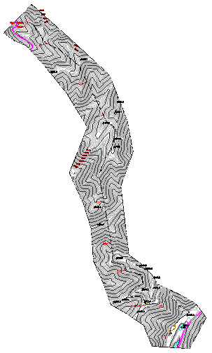
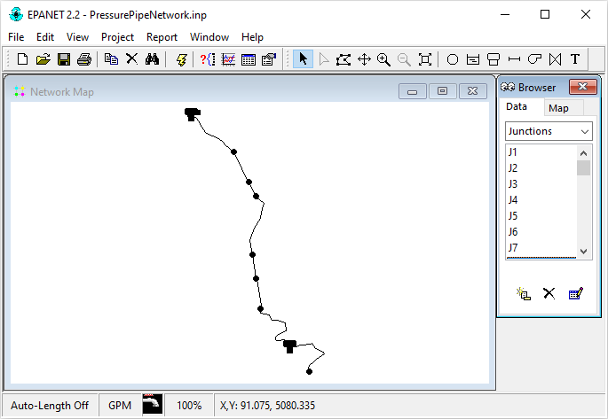
   This project contains a series of polylines that represents the pressure pipe network we are designing.
3. The drawing entities for the design surface that we will use to model drainage have already been prepared. These entities consist of design contours. Issue the Surface -- Triangulate & Contour command to display a dialog box similar to that shown below:
   

   Triangulate & Contour

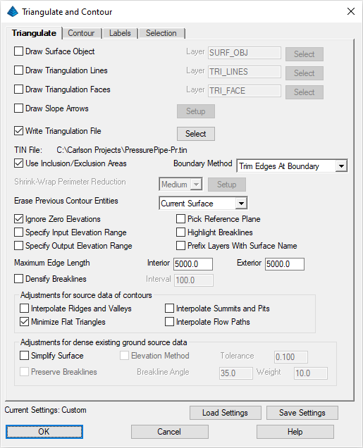
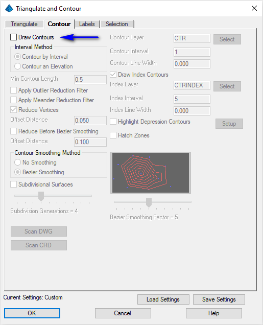
   Triangulate Tab	Contour Tab

   
   NOTE: Use the Select button on the Triangulate to create an output TIN file as illustrated above.
   Once set, click the OK button and when prompted:
   
   Select Inclusion perimeter polylines or ENTER for none.
   [FILter]/<Select entities>: pick the boundary polyline
   [FILter]/<Select entities>: press Enter
   Select Exclusion perimeter polylines or ENTER for none.
   [FILter]/<Select entities>: press Enter
   Select points and breaklines to Triangulate.
   [FILter]/<Select entities>: type ALL and press Enter
   [FILter]/<Select entities>: press Enter
   
   The surface representing proposed conditions is written.
4. Let's create a pressure pipe network file from the geometry presented. Issue the Network -- Pressure Pipe Network command to display a dialog box similar to that shown below:
   
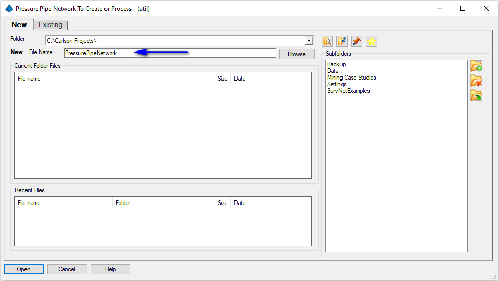
   Set the file name as illustrated above and click the Open button to display a "docked" dialog box as shown below:
   
5. We'd like to establish some initial, default settings for the project. Click the Settings (Gear) button to display a dialog box similar to that shown below:
   
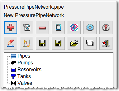
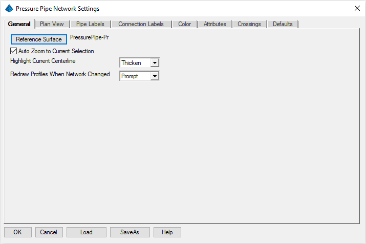
   Click the Reference Surface button to select the TIN file created earlier and then click the OK button.
6. For this example, zoom in to the upper left start of the pipe run so that we can select a small segment for our pump. The display should look like the following:
   
   Click the Add (Plus) button from the Network Actions row to display a dialog box similar to that shown below:
   
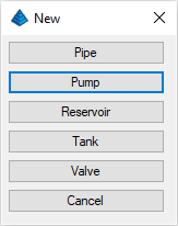
   To create a new pump, click the Pump button and the following dialog will appear:
   
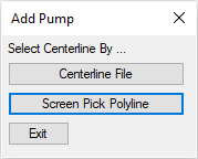
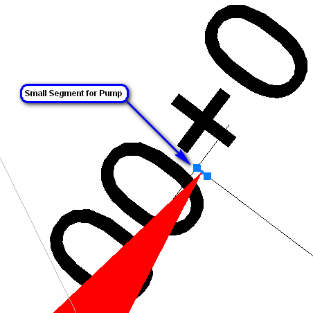
   For this example, click the Screen Pick Polyline button and when prompted:
   
   Select centerline polyline: pick the small polyline segment
   
   NOTE: Make sure the small segment is selected and not the longer pipe polyline.
   After selecting the small segment, the following dialog will appear:
   
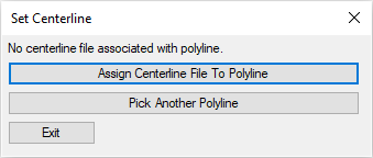
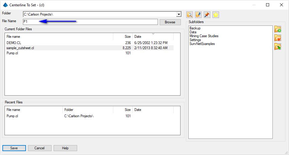
   Click the Assign Centerline File to Polyline to display a dialog box similar to that shown below:
   
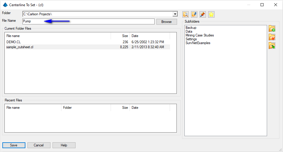
   Set the file name as shown above and click Save when ready. Upon creation of the centerline file, a dialog box similar to that shown below appears:
   
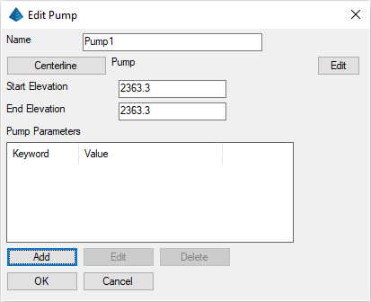
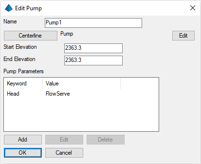
   Set a name for the pump as suggested above and also set the Start Elevation and End Elevation to 2363.3 (the surface model elevation at the pump location). The next step is to add the required pump parameters. Click the Add button and the following dialog box will appear:
   
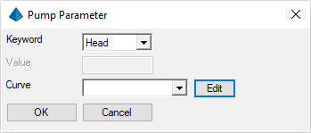
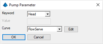
   Select the Head keyword and the Value field will be disabled and the Curve field will be enabled. To create a new pump curve, click the Edit button and the following dialog will appear:
   
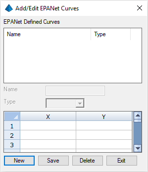
   This dialog allows for the entry of any one of the four EPANet Curves:
   1. Pump
   2. Efficiency
   3. Volume
   4. Headloss
   Click New and a new table will be created with a default name of NewCurve01:
   
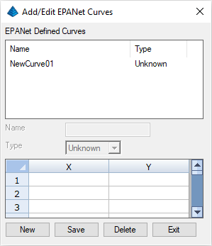
   Select the NewCurve01 entry and enter a new name of FlowServe and enter the following X, Y values:

   FlowServe Pump Curve Parameters

   Entry #	X (Head) Value	Y (Flow) Value
   1	250	810
   2	300	800
   3	350	795
   4	400	785
   5	500	750
   6	600	700
   7	700	640
   8	800	575

   The result should look similar to that shown below:
   
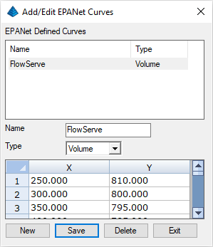
   Click the Save button and then click Exit to return to the Pump Parameter dialog box. Select the pump curve you created in the Curve field as illustrated below and click OK when ready:
   
   The Edit Pump dialog box should look as follows:
   
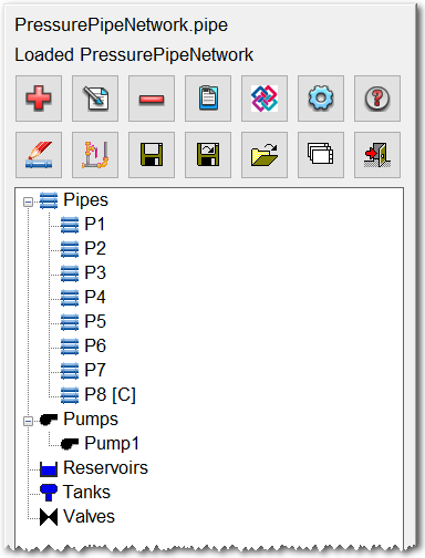
   Click OK to return to the docked dialog box which should look as follows:
   
7. To add a new pipe, either:
   • Click the Add (Plus) button on the Network Actions row and choose the Pipe option, or
   • Right-click on the Pipes category in the tree-view list and choose the Add Pipe option
   Do either option now to display the dialog box similar to that shown below:
   
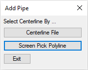
   For this example, click the Screen Pick Polyline button and when prompted:
   
   Select centerline polyline: pick the Pipe 1 polyline segment
   
   A dialog box similar to that shown below appears:
   
   Press the Assign Centerline File to Polyline to display a dialog box similar to that shown below:
   
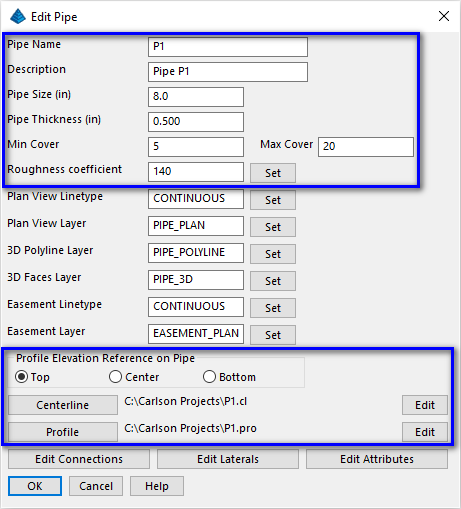
   Set the filename as shown above and click Save when ready to display a dialog box similar to that shown below:
   
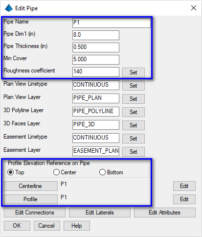
   Update the following values:
   • Pipe Dim 1 to 8.0
   • Pipe Thickness to 0.500
   • Min Cover to 5.0
   • Roughness Coefficient to 140
   • Profile Elevation Reference on Pipe to Top
   Additionally, click the Profile button to open a dialog box similar to that shown below:
   
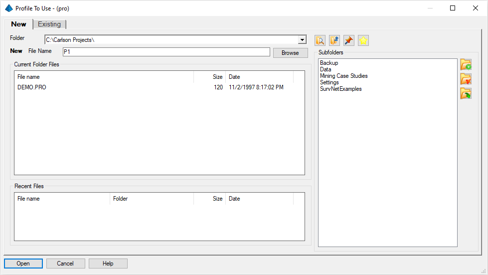
   Set the profile file name to be the same as the centerline name cited earlier and click Open when ready. Click OK to dismiss the Edit Pipe dialog box and add the pipe to the tree-view collection.
   
   Repeat the process of adding pipes for all eight pipes and use the same parameters for each pipe.
8. Pipe P8 has an required outflow of 600 cfs. To enter the demand, right-click on pipe P8 and click its Edit Pipe option. On the Edit Pipe dialog box, click the Edit Connections button at the bottom of the dialog to display a dialog box similar to that shown below:
   
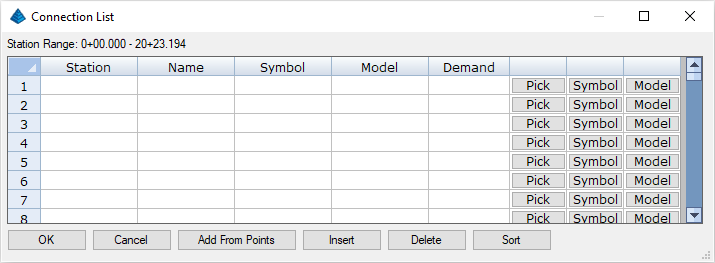
   Enter the End Station value 2023.194 which is displayed at the top of the dialog. The remaining values should be as shown in the following:
   
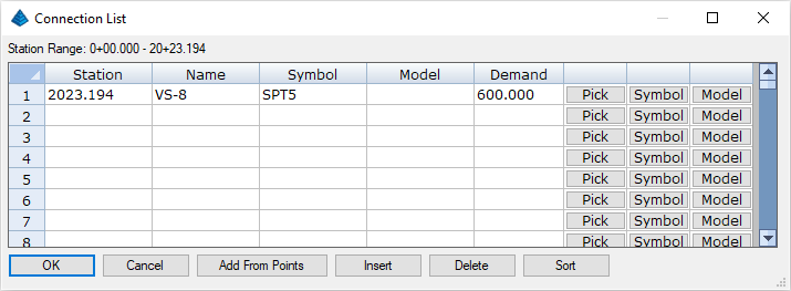
   Click OK to dismiss the Connection List dialog box and click OK to dismiss the Edit Pipe dialog box. The docked dialog should now look like the following:
   
9. In this example, we have two tanks. The Upper Tank and the Lower Tank as indicated on the drawing. To add a new tank, right-click the Tanks category in the tree-view and click the Add Tank button to display a dialog box similar to that shown below:
   
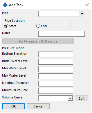
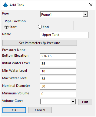
   The Pipefield contains a list of pipes, pumps, and valves that are currently defined in the project. For the Upper Tank, select the pump created earlier and indicate the tank is at the Start of the pump. Enter the remaining tank parameters as follows and click OK when ready:
   
   Repeat the process and add the second Lower Tank with the following parameters and click OK when ready:
   
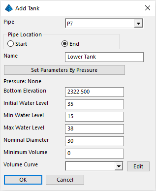
   NOTE: The Lower Tank is located to be at the End of P7.
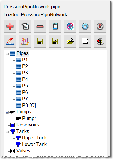
   The docked dialog should now look like the following:
   
10. Now that the model has been developed, an analysis can be performed. Click the EPANet (Pipes with Valve) button on the Network Actions row and the following dialog box will be displayed:
    
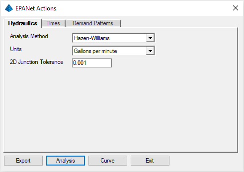
    Set the values as shown above and click the Analysis button to run the analysis which displays the results in the Standard Report Viewer similar to that shown below:
    
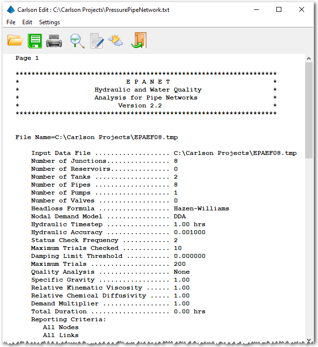
    Click the Exit (Doorway) to dismiss the report.
11. Click again on the EPANet button and click its Export button to create an EPANet input (*.inp) file which can be loaded via the EPANet via its File -- Import -- Network command:
    
    Click the Exit (Doorway) to dismiss the docked dialog box.

This completes the tutorial: Pressure Pipe Network Design.