
You may Remove or Edit files with the respective buttons. Individual settings may be modified directly in the spreadsheet of the main dialog.
Clicking the Add Row button will copy the currently selected block model, but the settings should be reviewed to ensure each model has a unique file name.
Clicking the Move Up/Down buttons will move the selected block model up/down in the list. This will change the order in which the block models are calculated.
Clicking the Clear button will delete all rows from the spreadsheet.
Clicking the Run button will generate the block model(s) in the list. The block model files will not be generated prior to clicking this button. Note that any files that have the Process column set to "No" will not be created.
Block Model Settings
When a new block model is added to the list, you will first be
prompted to set the filename. After this, the below dialog will
appear.

Bed Name: This list will only be populated by beds with
attributes. Note that bed names represent a collection of strata.
When a block model is created from a bed, there will be no
distinction of strata types unless the Model by Strata Name
option is enabled. In the above example, four beds with quality
attributes have been detected: OB and three distinct groups of LS.
You may select multiple beds for the block model, but it is
important to note that the block model will not keep track of the
bed name in the blocks. Only data points from the selected bed will
be used for block estimation. If more than one bed is selected,
there will be no distinction between the source of the data (in the
above example, the program will mix LS1, LS2, and LS3 data
points).
Attribute Name(s): This list shows the attributes
detected within the selected bed. You may include multiple
attributes in a single block model by clicking and dragging within
the list or by holding the CTRL key while selecting
attributes.
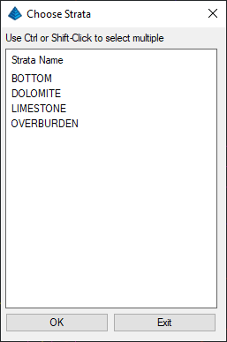
Model By Strata Names: This option will create the block
model from selected strata names (strata will be selected on the
following dialog). Note that Bed Names do not have to be listed in
order to model by Strata Names. This option will tag each block in
the model as having a different Strata Index number. For example,
Limestone blocks may be tagged with a 1, Clay blocks may be tagged
with a 2, Overburden blocks may be tagged with a 3, etc. This
allows you to distinguish between strata types in the block model
rather than simply grouping all blocks as part of the same bed. You
may still model quality attributes in the model when this option is
selected.
This option will automatically create a Grade Parameter File (.gpf file) that defines each Strata Index number. It is recommended to do this as it is the only place to keep track of the strata types in the block model. Note that the Grade Parameter File will have the same name as the Block Model, but will have a .gpf file extension.
This option will also automatically create a Geologic Model. This Geologic Model will be include a single layer with a block model added to define the variation in the qualities. When modeling by strata names, the block model actually defines the various types of strata, so it is not necessary to define multiple strata layers in the Geologic Model. Note that the Geologic Model will have the same name as the Block Model, but will have a .pre file extension.
When this option is enabled, the below dialog will appear after clicking OK. This dialog allows you to select the strata types to include in the block model. It is important to note that strata layers not selected will not be considered when the block model is created. For this reason, it is recommended to select all strata types in this list.

Horizontal Resolution Type: This option determines how the horizontal size of the blocks are defined. The Number of Block in X and Y option will use the X and Y fields to set the number of blocks in the horizontal plane. With this option, the dimensions of the cells will be calculated rather than manually set. The Block Dimensions option will set the block dimensions using the X and Y fields as the actual dimensions.
The XY extents of the block model may be set by clicking the Select Grid Position button. When this button is clicked, you will be prompted to select the corner extents of the block model.Vertical Position: This option will define the upper and lower bounds of the block model. The Fixed Elevations option will use flat elevations as specified by the Bottom Z and Top Z fields. The Follow Ore Model option will create grid files to define the upper and lower extents of the selected bed.
Crop Block by Estimated Strata/Bed: This option is only used when the Vertical Position is set to Fixed Elevation. When this option is off, the blocks will be populated with values at all elevations between the Top and Bottom Z. When this option is on, only some blocks will be populated with block values. The program will create top and bottom elevation grids that follow the ore layer, and any blocks outside of this elevation range will not be populated with values. To ensure that all blocks are populated with values, this option should be disabled.
Crop No Grade: This option is only available when using the Follow Ore Model option. When enabled, you will be able to specify a Grade Parameter File (.gpf file) to define the various grades of material. When making the upper and lower limits of the block model, these grids will only extend to portions of the bed that have been defined within the Grade Parameter File. In other words, any blocks with values not defined in the Grade Parameter File will be cropped out.
Selected Block Model Settings: This table lists various information about the extent of the block model to be created. Note that changing settings such as the Top/Bottom Z will cause this table to update.
After clicking OK, the below dialog will appear.

- The Discrete (Nearest Neighbor) method will use the nearest data point to of assign block values. No interpolation will be applied, but instead the block will take on the attribute value of the nearest sample point.
- The Kriging method will assign block values based on a
variogram. It is recommended to first calculate these variogram
parameters using the Geology Module > StrataCalc Pulldown Menu
> Calculate
Variogram command. When this option is used, you will be
prompted with the below dialog to set the kriging
parameters.

- The Inverse Distance method will use inverse distance weighting to assign block values. When this option is used, the below dialog will be displayed.

Maximum Inverse Samples: Sets the maximum number of data points to use when calculating the value of each block. The points nearest each block will be used for the calculation.
Minimum/Maximum Octant Samples: Sets the minimum/maximum number of data points to be used in each octant around the block to calculate the block value. If the program cannot detect the minimum number of data points in each octant, the block value will not be calculated.
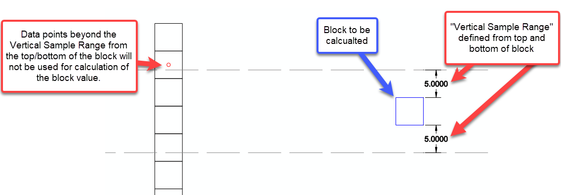
Vertical Sample Range: This option allows you to limit the vertical distance the program will search for data points when calculating block values. The below image is a visual explanation of this option with a Vertical Sample Range of 5. It is important to note that this Vertical Sample Range is checked as each individual block in the model is calculated.
Vertical Weight Factor: When using the Inverse Distance method as the modeling method, the Vertical Weight Factor can be used to modify the degree of vertical trending in the deposit. It should be noted that this value is not the same as the distance weighting power. When this value is set to 1.0, the model will be calculated using normal inverse distance weighting. When this value is greater than 1.0, the vertical distances between the blocks and the drillhole samples will be exaggerated by the Vertical Weight Factor to allow for more vertical variation in the model. When this value is less than 1.0, vertical variation in the model will decrease. The below diagram and table demonstrates how various Vertical Weight Factors will impact the relative weight of each sample on the resulting block value. In this example, an inverse distance weighting power of 2 is used for all calculations.
In the above example, there are 4 quality samples in the black drillhole. The example block lies 55' away from the drillhole at a centroid elevation of 100. Each of these 4 samples will be weighted to determine the actual value of the block. The table to the right shows how increasing the Vertical Weight Factor will impact the weight of each sample on the block value. Notice that as the Vertical Weight Factor increases, the weight of Sample 1 on the block value increases significantly, while the weight of Sample 4 on the block decreases significantly. This means that for a higher Vertical Weight Factor, a block's value will more closely resemble that of samples at elevations similar to the block.
The below images show how a block model can vary simply by modifying the Vertical Weighting Factor. Three values are used for comparison: 0.1, 1, and 10. Notice how the Vertical Weight Factor of 10 creates horizontal trending between the data points, whereas the other two model have decreasing degrees of horizontal trending. Note that when the Vertical Weight Factor is set to a low value of 0.1, there is almost no variation in the qualities in the vertical direction.

Search Radius: This value sets the search radius for the Inverse Distance modeling method. When the program is calculating the value of a block, any sample points further than this distance from the block centroid will be ignored.
Inverse Distance Power: Sets the weighting power for the inverse distance function. For more information on the Inverse Distance algorithm, see the Make Strata Grid File command documentation.
Use Ellipse Inverse Distance: This option will allow you to introduce a directional trend in the data. For example, if the data values tend to trend in a north-south direction (with more variation in the east-west direction), you may use an elliptical weighting factor.
Ellipse Azimuth: Sets the azimuth for the more heavily weighted data. For example, if data is expected to trend heavily in the north-south direction, an azimuth of zero should be used.
Ellipse Dip: Applies a dip to the anisotropic ellipse.
Ellipse Anisotropic Factor: The specified factor is used to increase the weight of data samples that line up more closely with the azimuth. Data samples that exactly line up with the azimuth apply additional weight, whereas data samples that are perpendicular with the azimuth apply zero extra weight. Data samples at an angle between the azimuth and perpendicular apply a proportional adjustment. The specified factor is adjusted by the azimuth and is then added with one and then multiplied by the data sample weight. For example, using an isotropic factor of 1 and a data sample that matches the azimuth to the model point, this sample will get double weighted; (1 + 1)*weight. When using a factor of 2 and a data sample that matches the azimuth, the sample will get triple weighted; (1 + 2)*weight.
Keyboard Command: BLKMODELAUTO
Pull-down Menu Location: Geology Module > Block Model