For each strata in the drillhole, this routine can generate 3D grid files of the strata thickness, top & bottom elevation, and attributes such as calcium, moisture, sulfur, and BTU. The grid files make up the geologic model in StrataCalc. A 3D grid file is a rectangular mesh of grid cells where each grid cell is the same size rectangle. The elevation or Z value of the four grid corners equals the value at those points. For example, consider a grid cell for a 3D grid mesh of strata thickness. The X and Y coordinates of a grid cell could be (0,0), (10,0), (10,15), and (0,15). The z values, which might be 4.5, 4.7, 4.8, and 4.6, represent the strata thickness at the four X and Y coordinates.
Make Strata Grid Files reads the strata data from the
drillholes. The strata data is correlated and processed for beds,
pinch out and conformance as specified in Carlson
Configure. The strata data points are then used with the
selected modeling method to calculate the grid. There is an option
to use a parameter file (made with Define Parameters) to filter the
strata data points. For example, when creating a thickness grid for
the overburden of 6_COAL, you could have a parameter filter of
THICKNESS 6_COAL > 1.0. This filter would make the program use
only drillholes with 6_COAL greater than 1.0 when calculating the
6_COAL overburden grid. See the Define Parameter File command for
more description on parameters.
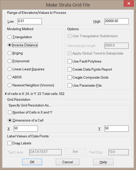
The routine starts by prompting for the location of the grid
files to create. The location can be specified by picking the lower
left and upper right corners or by selecting an existing grid file
which sets the new grid location and resolution to match the
selected existing grid file. Next there is the Make Strata Grid
File dialog for choosing the grid cell resolution, modeling method
and other parameters.
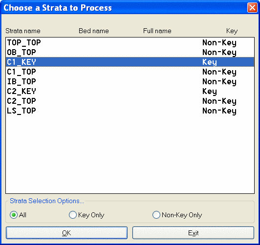
After the grid options dialog, the program prompts you to select the drillholes and fault lines. After reading in the selected drillholes, there is a Choose a Strata to Process dialog to choose the strata to process from the list. If Create Composite Grids was turned on, then multiple strata may be selected here. The All, Key Only and Non-Key Only are just viewing options to reduce the number of strata in the window if there are a lot, for ease of selection.
Then the program will prompt for the grid file name to create (.GRD). Next the program will process the strata data points to create the grid and the results are stored in a user-specified file name. The grids created by Make Strata Grid File can be used as the geologic model for the Geologic or Mining Model file. Also the grids can be used in the grid application routines, in the Civil Design module, such as Plot 3D Grid File, Grid File Utilities and Elevation Difference.
Making Strata Grids with Fault
Lines
There is an option to select fault lines in addition to the
drillholes. The fault lines should be drawn as 3D polylines with
elevations that equal the fault differential. The program will grid
with all modeling methods using the fault lines for making strata
elevation grids. The 3D fault polylines should be drawn such
that the left side of the polyline, relative to the direction of
the polyline, is the low side of the fault and the right side is
the high side. As each grid corner elevation is calculated, the
program checks each drillhole. If the drillhole is on the same side
of the fault polyline as the grid corner, then no adjustment is
made to the drillhole elevation data. Otherwise the drillhole is
projected onto the fault polyline and the polyline value at this
point on the polyline is used to adjust the drillhole elevation.
For example, if the fault polyline value was 5.0 and the grid
corner was on the high side of fault while the drillhole was on the
low side, then 5.0 would be added to the drillhole elevation
for modeling at that grid corner. If the grid corner was on the low
side and the drillhole was on the high side, then 5.0 would be
subtracted from the drillhole elevation. Reverse Polyline is
a good way to reverse the fault line if it is drawn in the wrong
direction.
Triangulation Modeling
Method
This method is straight triangulation between the drillholes.
Triangulation calculates these values by interpolating on the plane
defined by the three points in the triangle that encloses the
point. Since triangulation only interpolates, it can only calculate
values within the area of the data. Afterwards, an extrapolation
routine can then fill in the rest of the grid. This extrapolation
uses a safe method that tends to average out the data. There is an
option to extrapolation to apply the global trend. This option
finds the average slope and direction of the existing data and
applies this slope to extrapolating.
Inverse Distance Modeling
Method
Inverse distance calculates the grid values by assigning weights to
the existing data. The grid values calculated by inverse distance
are a weighted average of the existing data. Inverse distance will
not carry trends and the calculated grid values will never be
higher than the highest existing data point. Likewise the
calculated grid values will never be lower than the lowest existing
data point. The weights are proportional to the inverse of the
distance between the point to be estimated and the existing data
point. Closer points are weighted more than points farther away.
The inverse distance can be calculated to first, second, or third
power which are (1/d), (1/d^2), and (1/d^3) respectively. The power
can also be any user-specified number such as 2.5. The inverse
distance estimate is a weighted average with the individual weights
computed as an inverse power of distance as follows:
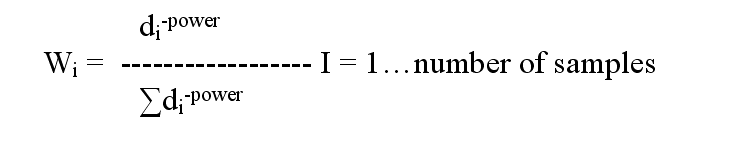
where Wi is the weight computed for each sample i, each di is
the distance between the location being estimated and sample I ,
and –power is the inverse distance weighting power.
In Configure under Mining there are several options for controlling
inverse distance. The Inverse Distance Search Radius is used for
calculating a value at a point such that only drillholes that are
within this Search Radius will be used in the calculations. The
Inverse Distance Max Samples value limits calculations to the
nearest specified number of drillholes to the point. For example,
the program will use the nearest 10 drillholes. Inverse distance
can also be controlled by quadrants which are divided into
northeast, southeast, southwest and northwest. The Min Quadrants
setting will use at least this specified number of drillholes from
each quadrant as long as there are drillholes in the quadrant
within the Search Radius. For instance, a setting of Min Quadrants
of one would make the program look for at least one drillhole from
each quadrant. The Max Quadrants value limits the number of
drillholes used from each quadrant. For example if Max Samples was
set to 25 and Max Quadrants was 10, then the total samples would be
25 with no more than 10 of the closest ones from each quadrant.
Elliptical inverse distance modeling method is an option that appears any time the Inverse distance modeling method is chosen. Elliptical inverse distance modeling will produce oval shaped model "bulls eyes" that are aligned by the specified azimuth of anisotrophy. The specified factor is used to increase the weight of data samples that line up more closely with the azimuth at the model point. Data samples that exactly line up with the azimuth apply the full factor. Data samples that are perpendicular with the azimuth apply zero extra weight. Data samples at an angle between the azimuth and perpendicular apply a proportional adjustment. The specified factor is adjusted by azimuth is then added with one and then multiplied by the data sample weight. For example, using a factor of 1 and a data sample that matches the azimuth to the model point, this sample will get weighted double; (1 + 1)*weight. When using a factor of 2 and a data sample that matches the azimuth, the sample will get weighted triple; (1 + 2)*weight. The prompts will appear:
Use inverse distance to which power
[First/<Second>/Third/Other]? Second
Use elliptical inverse distance [Yes/<No>]? Yes
Enter azimuth of anisotrophy: 45
Enter anisotropic factor: 1
With these values of
azimuth 45 and factor of 1, data samples that are NE/SW of the
model points will get double weight (1+1), data samples that are
NW/SE will get no extra weight, and data samples at in between
angles will get a proportional extra weight.
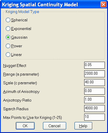
Kriging Modeling
Method
Kriging estimates the grid values by figuring the relationship
between all the existing data points and then assigning weights to
this data. Kriging finds the best fit linear unbiased estimates for
the given data and model. Kriging can carry trends within and
beyond the limits of the data and can find new high and low values.
You must supply a model that defines the spatial relationship of
the data which can be difficult. In fact, Kriging is a very
complicated subject and you will need to reference an outside
source for a detailed description such as An Introduction to
Applied Geostatistics by Isaaks and Srivastava. Carlson uses
Ordinary Kriging. All the parameters for this Kriging are specified
in the dialog shown.
Polynomial Modeling
Method
The polynomial method is based off of triangulation. The difference
is that instead of directly interpolating within each triangle, the
polynomial method creates smooth transitions by using a fifth
degree polynomial function that accounts for neighboring triangles.
Since polynomial needs adjoining triangles, when there are fewer
than five data points, there will be fewer than four triangles and
the polynomial method will revert to straight triangulation. The
same extrapolation logic for triangulation applies to the
polynomial method.
Linear Least Squares Modeling
Method
The linear least squares method finds the least squares best fit
plane at each grid corner. The least squares routine weights each
data point by inverse distance so that closer points are weighted
more than points farther away. So the best fit plane varies at
different points on the surface. The linear least squares method
extrapolates trends very well. A lower inverse distance factor
(i.e. 1.0) will weigh the data points more equally which models the
trends more globally (sometimes called "global dip"). Likewise a
higher inverse distance factor (i.e. 3.0) will weigh the closer
data points more heavily which models local trends strongly
(sometimes called "local dip"). Least squares will trend and allows
for data points that are new highs and lows, that don’t appear in
the original drillhole/point data. It does produce very nice,
smooth contours that honor the data points.
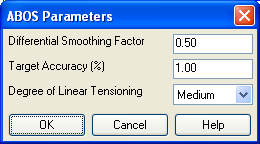 Differential Smoothing Factor:
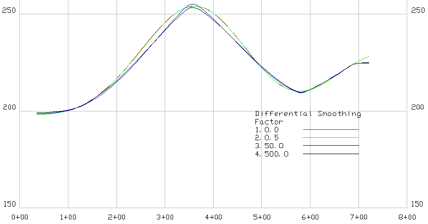

Use position from another file or pick grid position
(File/<Pick)? press Enter Using the position of an
existing file copies the grid resolution and corner point locations
to the new grid files. This is useful if you need to have grid
files match exactly. Most of the time, grids should match position
in the geologic model.
Pick Lower Left grid corner: enter or pick a
point
Pick Upper Right grid corner: enter or pick the second
point to define the grid position
Make Strata Grid File dialog box
Set the grid resolution and other options. A higher grid resolution
increases the processing time. Also choose the Modeling Method in
this dialog.
Select drillholes, channel samples and strata polylines.
Select objects: select the drillhole symbols
Select fault lines or Enter for none.
Select objects: press Enter for none, or select the fault
lines
Choose Strata to Process dialog
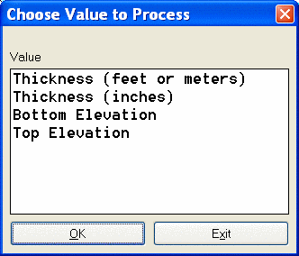
Choose Attribute to Process dialog
Pulldown Menu Location: StrataCalc
Keyboard Command: chgrid
| Converted from CHM to HTML with chm2web Standard 2.85 (unicode) |