- If you get the Start Page, pick Open Files.
- If you get the Startup Wizard dialog box, click the Browse button.
- If you are taken directly into CAD, click File -- Open.
Select entities for the scene.
[FILter]/<Select entities>: type ALL and press Enter twice
Here is a resulting graphic:
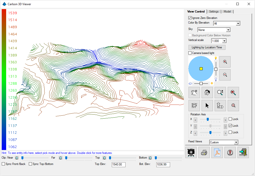
Click Exit (the doorway button) when finished.
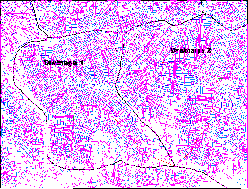
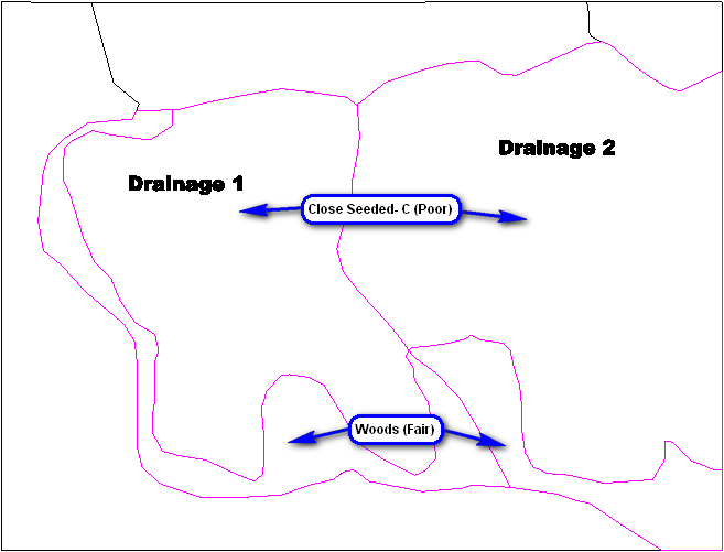
There are two main drainage areas that we will be looking at:
- Drainage 1
- Drainage 2
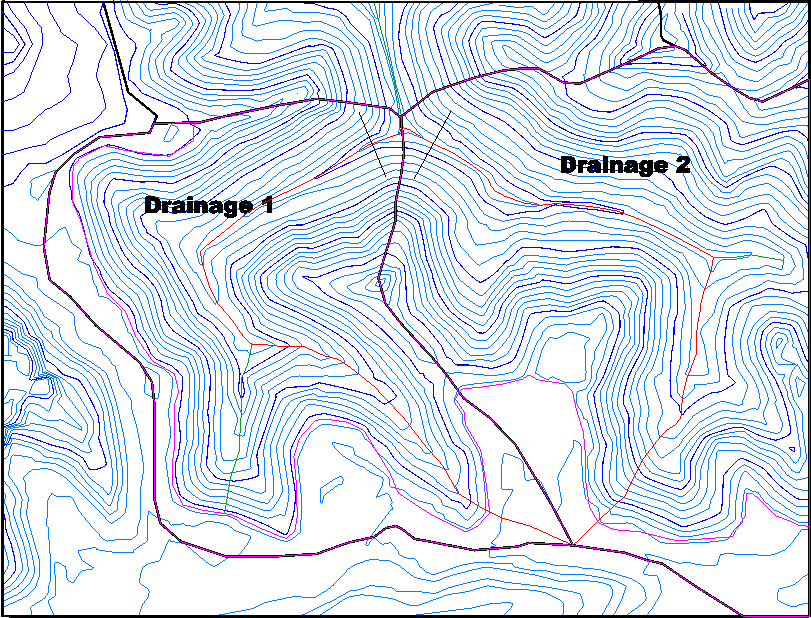
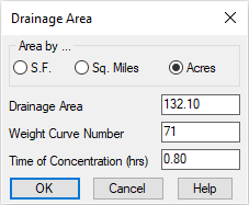
There are routines for finding these watersheds based on grid (*.grd) or TIN files, but this drawing has the closed polylines already generated. We will walk through some of the steps to gather the slope and area information.
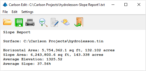
We would next like to evaluate the terrain data within each of the two watersheds available to us. Issue the Surface -- Slope Report command which displays the dialog box below:
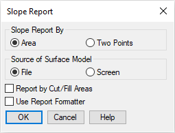
Set the values as shown above and click the OK button. On the subsequent dialog box, select the surface shown below and click the Open button when ready:
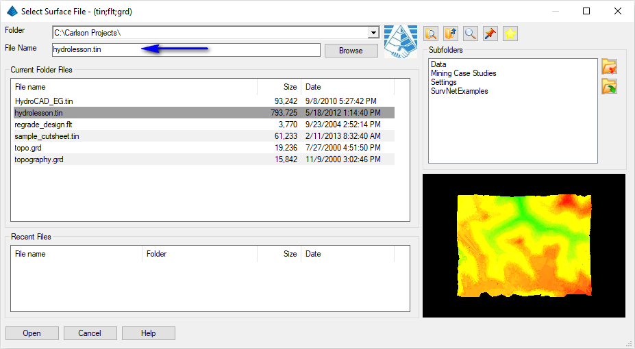
When prompted:
Select entities for the scene.
Select the Inclusion perimeter polylines or ENTER for none.
[FILter]/<Select entities>: select the closed perimeter line that runs around Drainage 1 (press Enter when complete)
Select the Exclusion perimeter polylines or ENTER for none.
[FILter]/<Select entities>: press Enter
The surface information from the selected TIN that is enclosed by the watershed perimeter polyline is echoed to the Standard Report Viewer as shown below:
 Click the
Exit (Doorway) button when finished. Immediately
press Enter to re-run the command and this time,
select the closed perimeter line that runs around Drainage
2. Contrast its results to that shown above:
Click the
Exit (Doorway) button when finished. Immediately
press Enter to re-run the command and this time,
select the closed perimeter line that runs around Drainage
2. Contrast its results to that shown above: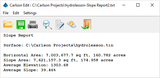
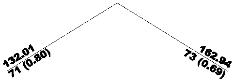
Notice that the watersheds are similar in size, and have approximately the same average slope. Click the Exit (Doorway) button when finished. Use the View -- Thaw/On All Layers command to thaw the layers that you froze earlier.
On the following dialog box, accept the parameters as shown below and click OK when ready:
The result will be a collection of 3D polylines showing the path(s) water will take from a given rainfall intensity amount. Among other things, the command is useful to fine-tune a watershed boundary. For example, the Pick Individually option can be used to spot-pick locations near a boundary line. You can see which direction the water will flow and adjust the watershed perimeter accordingly. Shown is an example of the drawing with the runoff tracking lines falling within their respective watersheds:
Issue the View -- Freeze Layer by Pick command and pick one of the previously generated flowlines and the two types of contour lines to remove them from the display.
Type of flow line [<3DPolyline>/Profile]? press Enter for the 3D Polyline option
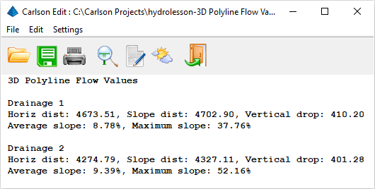
Select 3D polyline flow line: pick the Flowline for Drainage 1 as shown below
Select 3D polyline flow line: pick the Flowline for Drainage 2 as shown below
Select 3D polyline flow line: press Enter
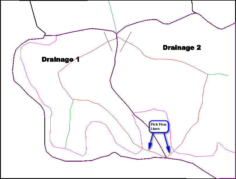
NOTE: The 3D polylines in the drawing were created (with runoff tracking and some editing) to represent the longest flow line.
The results are summarized in a nice report as illustrated below (with additional annotation added for clarity) showing the slopes and vertical drop. The report can be saved for future reference but "screen picks" of these polylines can be used in other aspects of the software:
Click the Exit (Doorway) button when finished.
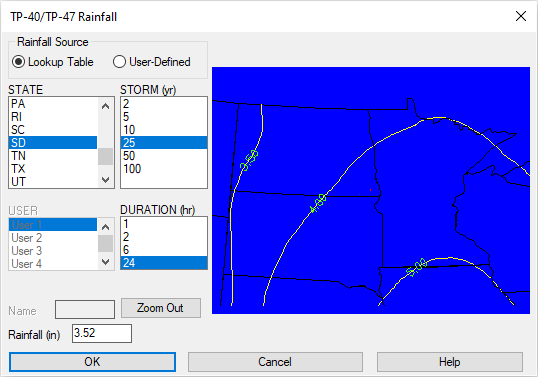
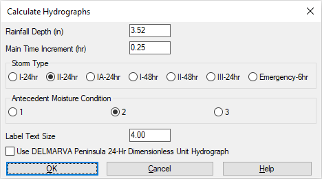
Set the values as shown above and note that as you click on the map, the rainfall intensity of the selected location will be reflected into the dialog box. For the sake of consistency, we will use the value of 3.52 inches (key this value in if you can't select it from the screen). For customizing this table to suit your needs, there is the User Defined toggle that permits individual entry in the lower left portion of the dialog box allowing for future retrieval if desired. Click OK when finished.
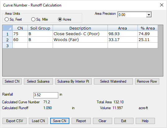
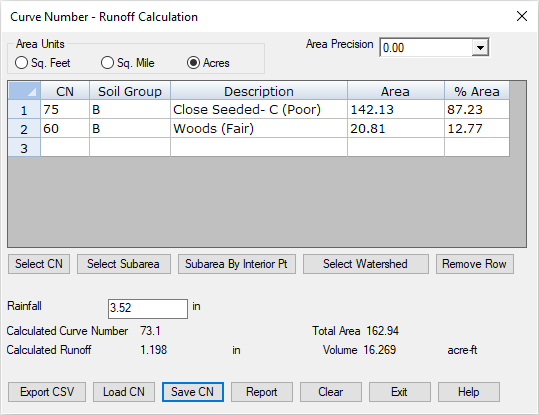
We will calculate a weighted curve number representing two land use types and will run this twice, once for each watershed. Issue the Watershed -- Curve Numbers (CN) & Runoff command. The following dialog box appears:
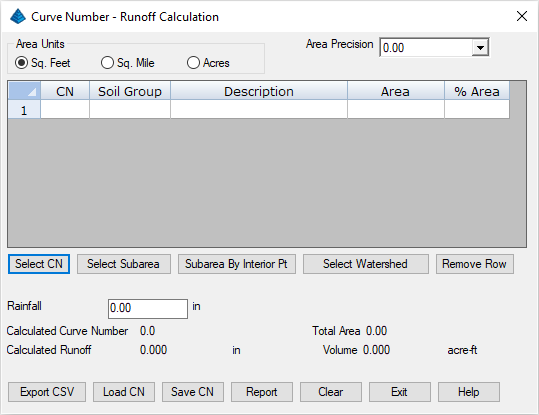
Let's specify the first of our two Curve Numbers. Click the Select CN button to display a dialog box similar to that below:
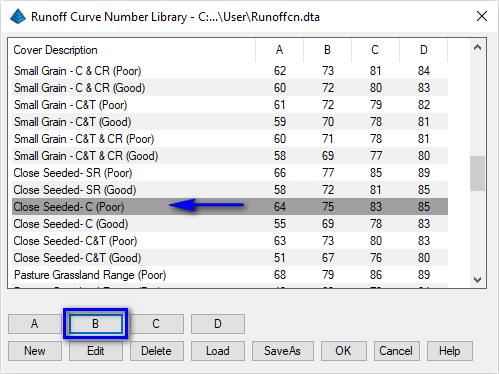
Scroll through the list to locate and highlight the Land Use cited above and then click soil type button B. The entry is loaded into the Curve Number - Runoff Calculation dialog box. Use the land use guide below for the exercise to follow:
With this entry active in the list, click the Subarea By Interior Point button and when prompted:
Pick point inside area perimeter: click within the Drainage 1 area for the land use identified as Close Seeded- C (Poor) as shown above
(the selected area will shade)
Use the Selected Area? click Yes when you have the correct watershed sub-area
Pick point inside area perimeter (Enter to end): press Enter
Let's specify the second of our two Curve Numbers. Highlight/select the empty Row 2, and click the Select CN button to display a dialog box similar to that below:
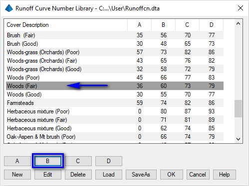
Scroll through the list to locate and highlight the Land Use cited above and then click soil type button B. The entry is loaded into the Curve Number - Runoff Calculation dialog box. Again, with the Row 2 entry active in the list, click the Subarea By Interior Point button and when prompted:
Pick point inside area perimeter: click within the Drainage 1 area for the land use identified as Woods (Fair) as shown above
(the selected area will shade)
Use the Selected Area? click Yes when you have the correct watershed sub-area
Pick point inside area perimeter (Enter to end): press Enter
Set the remaining values as shown below:
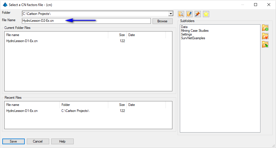
 Click on the
Save CN button to save this weighted Curve Number
data to a file as shown below:
Click on the
Save CN button to save this weighted Curve Number
data to a file as shown below: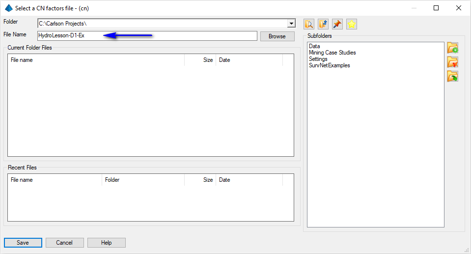
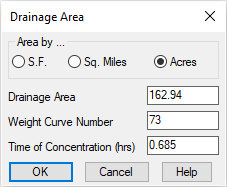
To obtain the weighted Curve Number for the Drainage 2 area, select/highlight the desired row/land use entry and click the Subarea By Interior Point button. Repeat for the other land use and the results should resemble that shown below:
Click on the Save CN button to save this weighted Curve Number data to a file as shown below:
Control returns to the Curve Number - Runoff Calculation dialog box and click the Exit button to complete the command.
NOTE: The CN number from the previous exercise (for Drainage 2) will be considered "active" and we'll need to exercise care to make sure the proper flowline is selected. Let's follow the Drainage 1/Drainage 2 process to make sure!
- Recall the Curve Number information for Drainage 1 by re-issuing the Hydrology -- Curve Numbers (CN) & Runoff command.
- Click the Load CN to load the *.cn file as
illustrated below (use the Open button rather than
the button shown here):
- Click the Exit button.
- Issue the Watershed -- Time of Concentration (Tc) --
SCS Method command. This will launch the Time of
Concentration (SCS) dialog box similar to that shown
below:
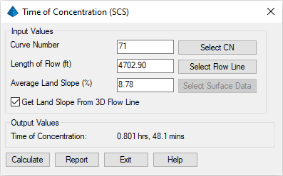
- Click the Select Flow Line button and
graphically select the Red flowline that contributes to
Drainage 1:
- With the settings shown, click the Calculate
to obtain the Tc for Drainage 1:
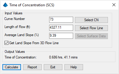
Note the two results and click Exit when ready.
- the View -- Freeze Layer by Pick command to leave the Watershed_Perim layer visible and follow with the Select Area from Screen button, or
- keying-in the value as reported in the Curve Number Runoff Calculation 1 exercise from above
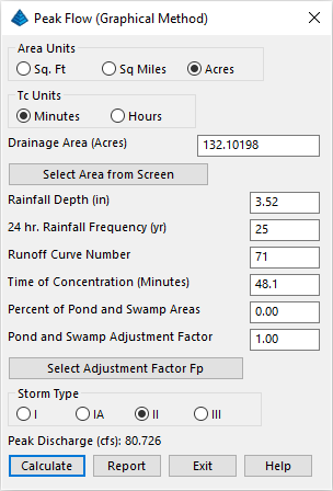
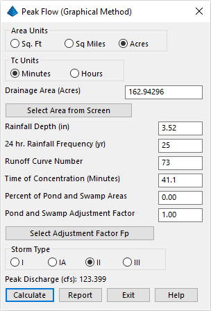
| Variable | Drainage 1 | Drainage 2 |
|---|---|---|
| Drainage Area (Acres) | 132.10198 | 162.94296 |
| Rainfall Depth (Inches) | 3.52 | 3.52 |
| 24 hr. Rainfall Frequency (Year) | 25 | 25 |
| Runoff Curve Number | 71 | 73 |
| Time of Concentration (Minutes) | 48.1 | 41.1 |
| Percent of Pond and Swamp Areas | 0.00 | 0.00 |
| Pon and Swamp Adjustment Factor | 1.00 | 1.00 |
| Storm Type | II | II |
| Peak Discharge | 80.726 | 123.399 |
| Drainage 1 | Drainage 2 |
|---|---|
|
|
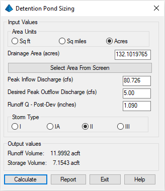
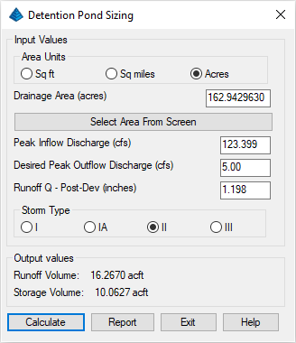
The Drainage Area and Peak Inflow Discharge values from the last area calculated will appear. In this example, we will allow for a combined maximum 10 ft³/sec (cfs) to be discharged from the ponds combined (in other words, 5 cfs from each will be our Desired Peak Outflow). Use the summary of values below and click Calculate. The Runoff Volume and the Storage Volume will appear at the bottom of the window:
| Variable | Drainage 1 | Drainage 2 |
|---|---|---|
| Drainage Area (Acres) | 132.10198 | 162.94296 |
| Peak Inflow Discharge (cfs) | 80.726 | 123.399 |
| Desired Peak Outflow (cfs) | 5.00 | 5.00 |
| Runoff Q - Post-Dev (inches) | 1.090 | 1.198 |
| Storm Type | II | II |
| Drainage 1 | Drainage 2 |
|---|---|
|
|
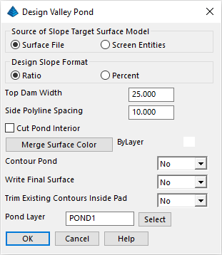
When prompted:
Pick top of pond polyline: pick the polyline for the Drainage 1 region
Select Existing Surface: specify the TIN file shown below and click the Open button when ready:
Pick point within pond: pick within the storage area (southwest of the dam centerline for Drainage 1)
Outslope ratio <2.00>: press Enter
Interior slope ratio <2.00>: press Enter
Top of dam elevation: 1109
Calculate stage-storage values [<Yes>/No]? press Enter
Method to specify storage elevations [<Automatic>/Interval/Manual]? specify the Interval (i) method
Starting elevation <1078.65>: 1078 (we'll start just below the lowest elevation)
Elevation interval <2.00>: press Enter (notice the Storage capacity of the pond is greater than the desired Storage Volume, click the Exit (Doorway) button when ready)
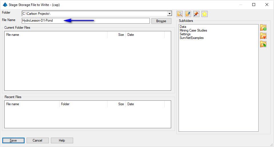
Write stage-storage file [Yes/<No>]? indicate Yes (indicate the file name below and click Save when ready)
Adjust parameters and redesign pond [Yes/<No>]? press Enter
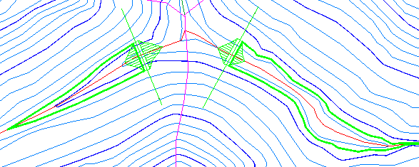
You should now have a pond that looks like the one on the left in the following image (emphasis added for clarity):
Repeat the routine for Pond 2 using the same parameters except:
- Top of dam elevation: 1087
- Starting elevation <1063.01>: 1062
- Write stage-storage file
[Yes/<No>]? indicate Yes
(indicate the file name below and click Save when
ready)

| Drainage 1/Pond 1 | Drainage 2/Pond 2 |
|---|---|
|
|
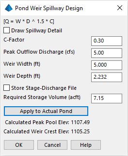
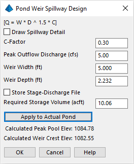
- C-Factor: 0.30
- Peak Outflow Discharge (cfs): 5.00
- Weir Width (ft): 5.00 (the Weir Depth will be found, however, we'll use a Drop Pipe in Pond 1, and a channel in Pond 2)
- Required Storage Volume (acft): provide the respective values shown above
Click the Apply to Actual Pond button and choose the Pond 1 stage-storage capacity file created earlier. This should yield two elevations shown in the dialog: the Peak Pool Elevation and the Weir Crest Elevation (bottom of spillway). This will be our principal spillway. Our emergency spillway will be assumed to be 1.5 feet higher.
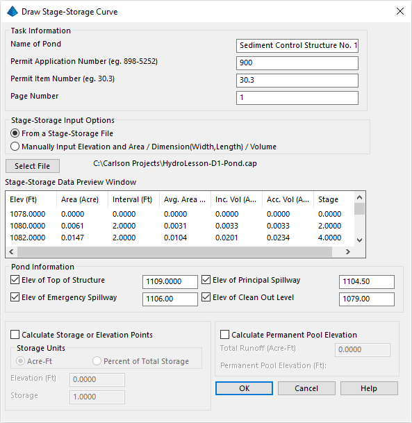
A secondary dialog box appears. Complete as follows and click OK when ready:
When prompted: Pick starting position: pick the lower left corner of the report
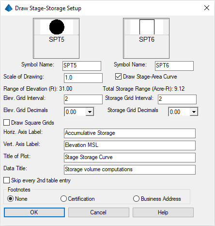
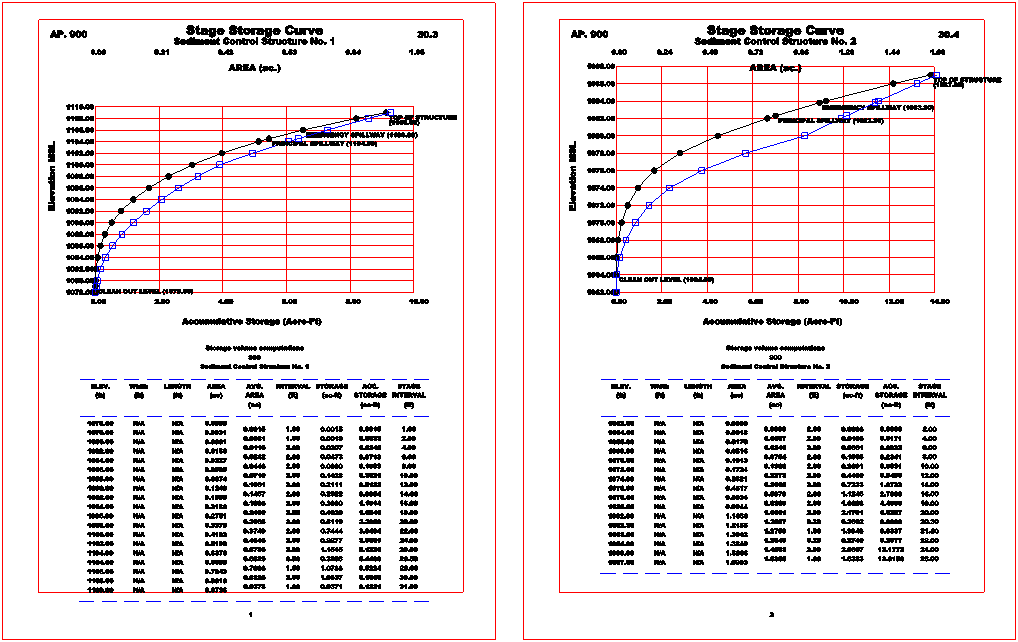
Do the same for Pond 2, with the other elevations from the Spillway and Top of dam as calculated above and choose to put this on Page Number 2. Your graphs should look like the two pictured below (emphasis added):
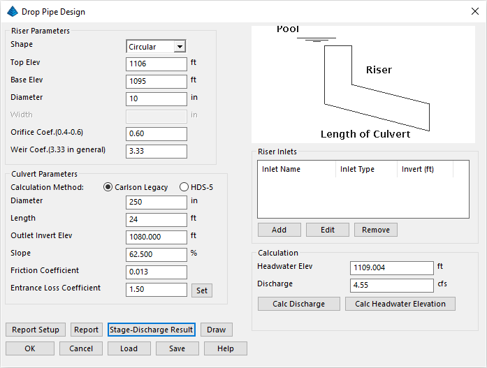
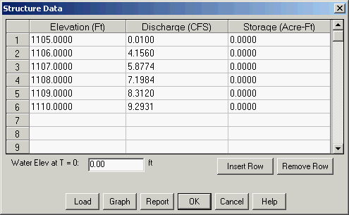
We will design one for the 5 cfs flow we need. Enter in the values shown in the window and click the Calc Discharge to see the results. We appear to be near the 5 CFS discharge we are looking for. Click the Stage-Discharge Result button to display a dialog box similar to that shown below and click OK when ready:
The results are summarized as illustrated below. Click the Write Stage-Discharge File button to create a *.stg file as suggested below:

Click Close and/or OK to dismiss any remaining dialog boxes.
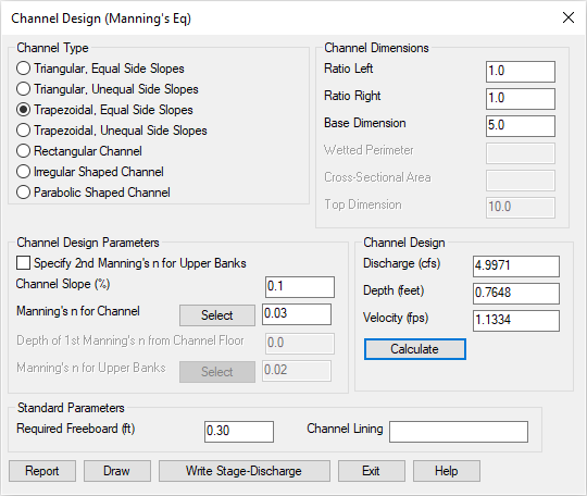
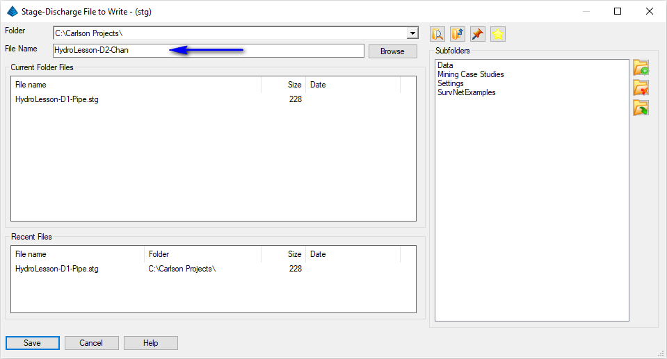
Specify the parameters shown except the Discharge (cfs) item... set its value to 5 and click on the Calculate button to determine the Channel Depth and Flow Velocity. Once satisfied, click on the Write Stage-Discharge button to create a *.stg file as suggested below and click Save when ready:
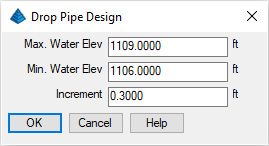
When prompted:
Maximum Depth <5>: 1.5
Interval <1>: 0.30
Base Elevation: 1082.30
Click Exit to dismiss the dialog box.
Issue the Watershed -- TR-20 Routing -- Draw Flow Polylines to approximate the direction of flow: As seen in the diagram, pick from SW to NE to simulate the general direction of flow for Drainage 1:
When prompted:
Text size <4.00>: press Enter
Draw from highest to lowest elevation (direction of flow).
Exit/Pick point: pick a starting location
Undo/Exit/Join/Pick point: pick an ending location to the northeast
Undo/Exit/Join/Pick point: press Enter and complete the values as shown and click OK when ready:
Draw another flow polyline [<Yes>/No]? press Enter
Exit/Pick point: pick a starting location
Undo/Exit/Join/Pick point: pick an ending location to the northwest
Undo/Exit/Join/Pick point: press Enter and complete the values as shown and click OK when ready:
Draw another flow polyline [<Yes>/No]? indicate No
When prompted:
Select flow polylines, structure and reach symbols.
[FILter]/<Select entities>: crossing Window the flow line entities and annotation
[FILter]/<Select entities>: press Enter
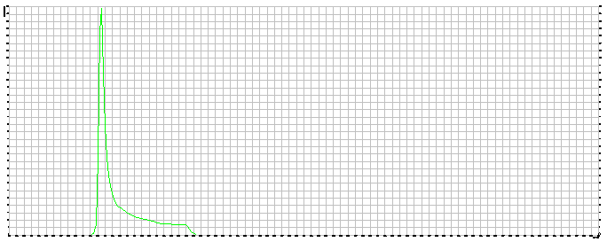
The routine will run TR-20 and give a Standard Report Viewer report. There are now some hydrograph files that we can draw in the next step.
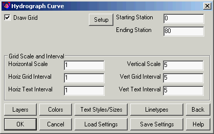
The scales to be used should be about 1,1,1,5,5,5 and we will draw the grid on the first one, and turn off the grid for additional hydrographs. Choose starting time of 0, and an ending time of 80 (the next one will go that long):
Click the Load button twice:
- once to pick the *.cap file, and,
- once again to pick the *.stg file