
The Processing buttons from left to right are:
Network Adjustment -
adjusts the network and creates a results report
Preprocess, compute
unadjusted coordinates - processes the network, calculates
positions and creates an error and coordinate report
Blunder Detection - processes the
network based on three user selected parameters and creates an
error report
Draw Network - draws the network in
an open CAD drawing based on the Drawing Settings set in the
Project
Settings

When you select Process -- Network Adjustment from the menu, the raw data will be processed and adjusted using least squares based on the Project Settings. If there is a problem with the reduction, you will be shown error messages that will help you track down the problem. Additionally a .ERR file is created that will log and display error and warning messages.
The data is first preprocessed to calculate averaged angles and distances for sets of angles and multiple distances. For a given setup, all multiple angles and distances to a point will be averaged prior to the adjustment. The standard error as set in the Project Settings dialog box is the standard error for a single measurement. Since the average of multiple measurements is more precise than a single measurement, the standard error for the averaged measurement is computed using the standard deviation of the mean formula.
Non-linear network least squares solutions require that initial approximations of all the coordinates be known before the least squares processing can be performed. So, during the preprocessing approximate coordinate values for each point are calculated using basic coordinate geometry functions. If there is inadequate control or an odd geometric situation, SurvNET may generate a message indicating that the initial coordinate approximations could not be computed. The most common cause of this problem is that control has not been adequately defined or there are point numbering issues.
Side-shots are separated from the raw data and computed after the adjustment (unless the "Enable sideshots for relative error ellipses" toggle is checked in the Adjustment dialog box). If side shots are filtered out of the least squares process and processed after the network is adjusted, processing is greatly sped up, especially for a large project with a lot of side shots.
If the raw data processes completely, a report file, .RPT, a .NEZ file, an .OUT file, and an .ERR file will be created in the project directory. The file names will consist of the project name plus the above file extensions. These different files are shown in separate windows after processing. Additionally, a graphic display of the network can be generated.
.RPT file: This is an ASCII file that contains the statistical and computational results of the least squares processing.
.NEZ file: This file is an ASCII file containing the final adjusted coordinates. This file can be imported into any program that can read ASCII coordinate files. The format of the file is determined by the ASCII NEZ setting in the Project Settings dialog box.
.OUT file: The .OUT file is a formatted ASCII file of the final adjusted coordinates suitable for display or printing.
.ERR file: The .ERR file contains any warning or error messages that were generated during processing. Though some warning messages may be innocuous it is always prudent to review and understand the meaning of the messages.
If you have "Write to Coordinate File" checked in the Output options dialog, the coordinates will also be written to a coordinate file (.CRD by default).
The following is an example of the initial report displayed in
the dialog box showing the calculation results.

GPS vector networks can be adjusted with SurvNET. This chapter will describe the processing of a simple GPS network. Following is a graphic view of the GPS network that is to be adjusted. Points A and B are control points. The magenta lines represent measured GPS vectors. Most GPS vendor's software can output GPS vectors to a file as part of the post-processing of GPS data.

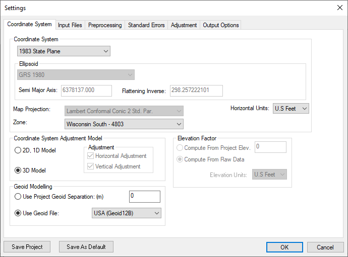
When processing GPS vectors, certain project settings are important. In the following settings dialog box, notice that the 3D-model has been chosen and SPC 1983 with the appropriate zone has been chosen. The 3-D model and a geodetic coordinate are required when processing GPS vectors. Though it is not required for GPS processing, it is in most cases appropriate to choose to do geoid modeling.
The following settings dialog box shows the raw files used in processing GPS files. A GPS vector file must be chosen. GPS vector files from various GPS vendors are supported. Select the vector files to be processed:

Coordinate control for the network can be in one of several files. The control can be located in the GPS vector file itself. More typically, the control points can be regular coordinate records in the .RW5 or the .CGR file. They also can be entered as 'Supplemental Control' in one of the available formats.
When the control coordinates are in the raw data file they are expected to be grid coordinates with orthometric heights.
The supplemental control file formats support grid coordinates with orthometric heights, geographic coordinates with orthometric heights, or geocentric coordinates with ellipsoid heights.
If the control coordinates are found in the GPS vector file, they are assumed to be Geocentric ECEF (earth-centered-earth-fixed) XYZ coordinates. As shown in the dialog above, it is not unusual to have different distance units for GPS, total station data, and control data. GPS vector data is usually in metric units but the total station raw file can be in US Feet. So, the distance units must be specified for the different raw data types.
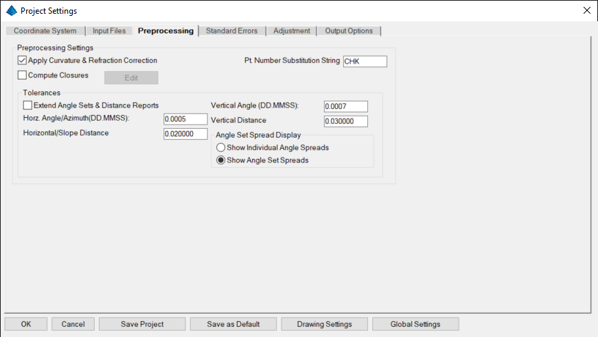
In the Preprocessing Settings dialog box, the only important setting is the Compute Closures option. If GPS loop or point-to-point closures need to be computed, the point numbers defining the loops need to be entered into a Closure File. See the discussion on traverse closures to see how to create Closure Files.
There are two GPS standard errors fields in the Standard Errors Settings dialog box. The GPS vector XYZ standard errors and covariances do not need to be defined as project settings since they are found in the GPS vector data files.
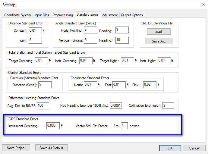
For more information, see the discussion on GPS Standard Errors.
Processing a GPS vector network together with conventional total station data is similar to processing a GPS network by itself. The only difference in regards to project settings is that a raw data file containing the total station data needs to be chosen as well as a GPS vector file. The project must be set up for the 3D model and a geodetic coordinate system needs to be chosen. The total station data must be 3D, all rod heights and instrument heights must be measured.
Following is a view of the Input Files Settings dialog box showing both a GPS vector file and a total station raw data file chosen in a single project. It is not uncommon to have different distance units for GPS data and total station data, so make sure the correct units are set for data types.

One of the most common problems for new users in combining GPS and total station data is not collecting HI's and rod heights when collecting the total station data. Since the 3D model is being used complete 3D data needs to be collected. If you only have 2D traverse data, you can adjust the GPS vectors first and then use the adjusted coordinates as control for the Traverse data project.

The 'Preprocess, Compute Unadjusted Coordinates' option allows the computation of unadjusted coordinates. If there are redundant measurements in the raw data, the first angle and distance found in the raw data is used to compute the coordinates. If a State Plane grid system has been designated the measurements are reduced to grid prior to the computation of the unadjusted coordinates. If the point is located from two different points the initial computation of the point will be the value stored.

A variety of blunder detection tools are available that gives the user additional tools in analyzing the survey data and detecting blunders. The standard least squares adjustment processing and its resulting report can often be used to determine blunders. No blunder detection method can be guaranteed to find all blunders. So much depends on the nature of the network geometry, the nature of the measurements, and the intuition of the analyst. Generally, the more redundancy there is in a network the easier it is to detect blunders.
There are three different methods that can be used to track down blunders in a network or traverse:
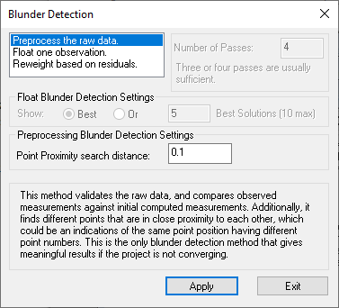
The Preprocess the raw data option validates the raw data. It displays angle and distance spreads as well as checks the validity of the raw data. Traverse Closures are computed if specified. It also performs a "K-Matrix" analysis. The "K-Matrix" analysis compares the unadjusted, averaged measurements with the computed preliminary measurements (measurements calculated from the preliminary computed coordinates). This method will catch blunders such as using the same point number twice for two different points. The report will be sent to the .ERR file. The .ERR file will contain the tolerance checks, closures and the K-Matrix analysis. Following is an example of the report created using the 'Preprocess the raw data' option. Notice that the first section of the report shows the angle and distance spreads from the multiple angle and distance measurements. The second part of the report shows the 'K-matrix' analyses.
Additionally there is a 'Point Proximity Report' section that reports pairs of different points that are in close proximity to each other which may indicate where the same point was collected multiple times using different point numbers.
The 'Preprocess the raw data' option is one of the simplest and effective tools in finding blunders. Time spent learning how this function works will be well spent. If the project is not converging due to an unknown blunder in the raw data, this tool is one of the most effective tools in finding the blunder. Many blunders are due to point numbering errors during data collections, and the 'K-matrix' analysis and 'Point Proximity' search are great tools for finding this type blunders.
     =====================================
     LEAST SQUARES ADJUSTMENT ERROR REPORT
     =====================================

Tue Mar 21 16:04:00
Input Raw Files:
    C:\Carlson Projects\cgstar\CGSTAR.CGR
Output File: C:\Carlson Projects\cgstar\cgstar.RPT

Checking raw data syntax and angle & distance spreads.

Warning: Missing Vert. Angle. Assumption made as to whether it is direct or reverse.
  1                                   5.00  180.00050                              4
Warning: Missing Vert. Angle. Assumption made as to whether it is direct or reverse.
  1                                   5.00  180.00070                              5
Warning: Missing Vert. Angle. Assumption made as to whether it is direct or reverse.
  1                                   5.00  180.00100                             10
Warning: Missing Vert. Angle. Assumption made as to whether it is direct or reverse.
  1                                   5.00  180.00020                             11
Warning: Missing Vert. Angle. Assumption made as to whether it is direct or reverse.
  1                                   5.00  325.54320                              2     H&T
Warning: Missing Vert. Angle. Assumption made as to whether it is direct or reverse.
  1                                   5.01  145.54300                              2     H&T
Warning: Missing Vert. Angle. Assumption made as to whether it is direct or reverse.
  1                                   5.01  180.00020                             12
Horizontal Angle spread exceeds tolerance:
  IP: 1,  BS: 5,  FS: 2
  Low: 109-19'10.0" ,  High: 109-19'17.0" ,  Diff: 000-00'07.0"

Horizontal Angle spread exceeds tolerance:
  IP: 2,  BS: 1,  FS: 6
  Low: 190-32'02.0" ,  High: 190-32'10.0" ,  Diff: 000-00'08.0"

Horizontal Angle spread exceeds tolerance:
  IP: 2,  BS: 1,  FS: 3
  Low: 096-03'48.0" ,  High: 096-03'56.0" ,  Diff: 000-00'08.0"

Horizontal Angle spread exceeds tolerance:
  IP: 3,  BS: 2,  FS: 4
  Low: 124-03'50.0" ,  High: 124-03'56.0" ,  Diff: 000-00'06.0"

Horizontal Angle spread exceeds tolerance:
  IP: 5,  BS: 4,  FS: 10
  Low: 039-26'35.0" ,  High: 039-26'45.0" ,  Diff: 000-00'10.0"

Horizontal Angle spread exceeds tolerance:
  IP: 10,  BS: 5,  FS: 11
  Low: 241-56'23.0" ,  High: 241-56'35.0" ,  Diff: 000-00'12.0"

Horizontal Angle spread exceeds tolerance:
  IP: 11,  BS: 10,  FS: 12
  Low: 114-56'20.0" ,  High: 114-56'34.0" ,  Diff: 000-00'14.0"

Horizontal Angle spread exceeds tolerance:
  IP: 12,  BS: 11,  FS: 3
  Low: 140-39'18.0" ,  High: 140-39'31.0" ,  Diff: 000-00'13.0"

Horizontal Angle spread exceeds tolerance:
  IP: 5,  BS: 4,  FS: 1
  Low: 117-30'35.0" ,  High: 117-30'50.0" ,  Diff: 000-00'15.0"

Horizontal Distance from 2 to 3 exceeds tolerance:
  Low: 324.15,  High: 324.20,  Diff: 0.04

Vertical Distance from 2 to 3 exceeds tolerance:
  Low: 6.62,  High: 8.36,  Diff: 1.74

Vertical Distance from 3 to 4 exceeds tolerance:
  Low: 11.46,  High: 11.51,  Diff: 0.05

Horizontal Distance from 12 to 3 exceeds tolerance:
  Low: 144.64,  High: 144.66,  Diff: 0.02


K-Matrix Analysis.

Distance: From pt.: 4  To pt.: 5
   Measured distance:    309.61  Initial computed distance:    309.65
   Difference:     -0.04

Distance: From pt.: 12  To pt.: 3
   Measured distance:    144.63  Initial computed distance:    144.66
   Difference:     -0.03

Distance: From pt.: 5  To pt.: 6
   Measured distance:    348.51  Initial computed distance:    523.29
   Difference:   -174.79

Angle: IP: 4  BS: 3  FS: 5
   Measured angle:          093-02'11.5"
   Initial computed angle:  093-01'45.1"
   Difference:  000-00'26.4"

Angle: IP: 12  BS: 11  FS: 3
   Measured angle:          140-39'24.5"
   Initial computed angle:  140-40'32.6"
   Difference: -000-01'08.1"

Angle: IP: 5  BS: 4  FS: 1
   Measured angle:          117-30'42.5"
   Initial computed angle:  117-31'16.4"
   Difference: -000-00'33.9"

Angle: IP: 5  BS: 4  FS: 6
   Measured angle:          145-30'34.0"
   Initial computed angle:  079-39'46.4"
   Difference:  065-50'47.6"

Point Proximity Report:

  Points  3  and 30 are within      0.05 of each other.
The problem with the above project was that point 6 was accidentally used twice for two separate side shots. Because of the point numbering problem the project would not converge, using the regular least squares processing. The 'Preprocess the raw data' option was then used. Notice in the K-matrix section the distance from 5 to 6 shows a difference of 174.79' and the angle 4-5-6 shows a difference of 065-50'47.6". Then notice that the other listed differences are in the range of .02' for the distances and less than a minute for the angles. This report is clearly pointing out a problem to point 6.
Note the point proximity report section. During data collection, point number 30 was used as the point number when the point was previously collected as point 3.
In the first section of the report, notice that there are several warnings concerning whether a horizontal angle reading was collected in direct or reverse reading. The preprocessing software uses the vertical angle reading to determine the angle face of the horizontal angle reading. If the vertical angle is missing, the program makes its best guess as to whether the angle was collected in direct or reverse face. Since all horizontal angle spreads in the report are reasonable, the preprocessing software must have made the correct determination.
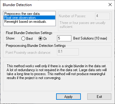
This option is useful in finding a single blunder, either an angle or distance, within a network or traverse. If there is more than a single blunder in the network then it is less likely that this method will be able to isolate the blunders. If the standard least squares processing results in a network that will not converge, then this blunder detection method will not work. Use the Preprocess the raw data blunder detection method if the solution is not converging. Also this method will only work on small and moderately sized networks. This method performs a least squares adjustment once for every non-trivial measurement in the network. So for large networks this method may take so long to process that it is not feasible to use this method.
With this method, an adjustment is computed for each non-trivial individual angle and distance measurement. Consecutively, a single angle or distance is allowed to float during each adjustment. The selected angle or distance does not "constrain" the adjustment in any way. If there is a single bad angle or distance, one of the adjustment possibilities will place most of the error in the "float" measurement, and the other measurements should have small residuals. The potentially bad angle or distance is flagged with a double asterisk (**). Since an adjustment is computed for each measurement, this method may take a long time when analyzing large data files.
The adjustments with the lowest reference variances are selected as the most likely adjustments that have isolated the blunder. You have the choice to view the best adjustment, or the top adjustments with a maximum of ten. In the above example, we asked to see the top 5 choices for potential blunders. The results are shown in the .ERR file. Following is a section of the report generated where an angular blunder was introduced into a small traverse. Notice the '**' characters beside the angle measurements. In this report the two most likely adjustments were displayed. The blunder was introduced to angle 101-2-3. Angle 101-2-3 was chosen as the 2nd most likely source of the blunder, showing that these blunder detection methods though not perfect, can be a useful tool in the analysis of survey measurements. Notice how much higher the standard residuals are on the suspected blunders than the standard residuals of the other measurements.
Adjusted Observations
=====================

Adjusted Distances
 From Sta.  To Sta.        Distance      Residual     StdRes.   StdDev
 101           2             68.780    -0.006         0.608    0.008
 2             3             22.592    -0.006         0.573    0.008
 3             4             47.694    -0.002         0.213    0.008
 4             5             44.954    -0.001         0.069    0.008
 5             6             62.604     0.005         0.472    0.009
 6             7             35.512     0.006         0.539    0.008
 7             101           61.704     0.003         0.314    0.009
            Root Mean Square (RMS)      0.005

Adjusted Angles
 BS Sta. Occ. Sta.  FS Sta.    Angle       Residual      StdRes    StdDev(Sec.)
 7          101      2        048-05'06"       -5          0          21
 101        2        3        172-14'33"       -2          0          27
 2          3        4        129-27'44"     -222   *      7          56   **
 3          4        5        166-09'59"       11          0          25
 4          5        6        043-12'26"       22          1          21
 5          6        7        192-11'52"       12          0          25
 6          7        101      148-38'19"        8          0          25
                               Root Mean Square (RMS)      85

Adjusted Azimuths
 Occ. Sta.  FS Sta.      Bearing           Residual    StdRes   StdDev(Sec.)
 101         7          N 00-00'00"
E            0             0            4
                Root Mean Square
 (RMS)          0

Statistics
==========

 Solution converged in 2 iterations
 Degrees of freedom:3
 Error Factors... (not shown)
 Standard error unit Weight: +/-0.88
 Reference variance:0.78
 Passed the Chi-Square test at the 95.00 significance level
 0.216 <= 2.347 <= 9.348


Adjusted Observations
=====================

Adjusted Distances
 From Sta.  To Sta.        Distance      Residual     StdRes.   StdDev
 101           2             68.781    -0.005         0.473    0.009
 2             3             22.592    -0.005         0.512    0.009
 3             4             47.690    -0.006         0.586    0.009
 4             5             44.950    -0.005         0.523    0.009
 5             6             62.605     0.006         0.607    0.009
 6             7             35.512     0.006         0.560    0.009
 7             101           61.708     0.006         0.614    0.009
            Root Mean Square (RMS)      0.006

Adjusted Angles
 BS Sta.  Occ. Sta.   FS Sta.    Angle        Residual      StdRes   StdDev(Sec.)
 7         101         2        048-05'22"       11           0        24
 101       2           3        172-11'03"     -213    *      7        58   **
 2         3           4        129-31'23"       -3           0        29
 3         4           5        166-09'48"        1           0        26
 4         5           6        043-12'11"        6           0        21
 5         6           7        192-11'50"       10           0        27
 6         7           101      148-38'24"       13           0        27
                               Root Mean Square (RMS)       81

Adjusted Azimuths
 Occ. Sta.  FS Sta.      Bearing           Residual    StdRes   StdDev(Sec.)
 101         7          N-00-00'00"E           -0             0            5
                Root Mean Square (RMS)          0

Statistics
==========

 Solution converged in 2 iterations
 Degrees of freedom:3
 Error Factors... (not shown)
 Standard error unit Weight: +/-0.94
 Reference variance:0.89
 Passed the Chi-Square test at the 95.00 significance level
 0.216 <= 2.675 <= 9.348
The blunder is most likely in the measurement containing the largest residual and standard residual. The observation marked with ** is the observation that floated. It is also most likely the measurement containing the blunder.
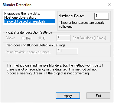
This method is capable of detecting multiple blunders but one is more likely to find the blunders if there is a high degree of redundancy (network of interconnected traverses). The higher the degree of freedom the more likely this method will find the blunders. This method will not work if the standard least squares processing will not converge. Use the Preprocess the raw data blunder detection method if the network is not converging.
First, select the number of adjustments or passes you wish to make. Each time an adjustment is completed, the measurements will be re-weighted based on the residuals and standard errors. Hopefully, after three or four passes, the blunders will become obvious. The results are shown in the .ERR file, look for the measurements with the highest standard residuals. These measurements are more likely to contain blunders.
The theory behind this method is that after processing, the measurements with blunders are more likely to have higher residuals and computed standard errors. So, in the next pass the measurements are re-weighted based on the computed residuals, with less weight being assigned to the measurements with high residuals. After several passes it is likely that the measurements with the blunders have been reweighed such that they have little effect on the network.
As a rule of thumb, three or four passes are usually sufficient. Following is a section of the report showing the results of the 'Reweight based on residuals'. This report was generated using the same data used in the earlier example. Notice that it has flagged the same two angle measurements.
The 'Reweight based on residuals' method performs a new adjustment for each pass. So, this method will take longer than the standard least squares adjustment, but does not take near as long to complete processing as the Float one Observation method for larger networks.
Adjusted Observations
=====================

Adjusted Distances
 From Sta.  To Sta.        Distance      Residual     StdRes.   StdDev
 101           2             68.778    -0.009         0.827    0.014
 2             3             22.588    -0.010         0.942    0.015
 3             4             47.694    -0.002         0.208    0.009
 4             5             44.954    -0.001         0.077    0.006
 5             6             62.608     0.010         0.919    0.016
 6             7             35.517     0.011         1.040    0.016
 7             101           61.705     0.004         0.398    0.011
            Root Mean Square (RMS)      0.008

Adjusted Angles
 BS Sta.  Occ. Sta.   FS Sta.       Angle          Residual    StdRes   StdDev(Sec.)
 7         101         2          048-05'07"        -4            0       21
 101       2           3          172-13'19"       -77     *      2       65
 2         3           4          129-29'56"       -91     *      3       64
 3         4           5          166-09'44"        -3            0       24
 4         5           6          043-12'05"         0            0        9
 5         6           7          192-11'40"        -0            0       19
 6         7           101        148-38'10"        -1            0       20
                               Root Mean Square (RMS)          45

Adjusted Azimuths
 Occ. Sta.  FS Sta.      Bearing           Residual    StdRes   StdDev(Sec.)
 101         7          N 00-00'00"E            0             0            2
                Root Mean Square (RMS)          0


Statistics
==========

 Solution converged in 1 iterations
 Degrees of freedom:3
 Error Factors... (not shown)
 Standard error unit Weight: +/-1.33
 Reference variance:1.77
 Passed the Chi-Square test at the 95.00 significance level
 0.216 <= 5.322 <= 9.348
The blunders are most likely in the measurements containing the largest residuals and standard residuals.
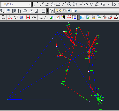
If you are running SurvNET from inside Carlson Survey with AutoCAD or IntelliCAD, you can draw the network in the DWG file. The Drawing Settings option located in the Settings Menu will determine the layers and symbols used for each point and line entity.
The Draw Network option will not be available until the network has been adjusted. After the adjustment, you can select Draw Network.

Your project will be drawn in the drawing (.DWG) file. Put focus back in the CAD program to view the network.
| Converted from CHM to HTML with chm2web Standard 2.85 (unicode) |