Surface Mine Reserves
This command calculates quantities and qualities directly from
drillholes or from predefined Geologic/Mining Models. Additional
outputs include stripping ratio contours, composite thickness
grids, and more. The dialog is divided into three tabs - Process,
Adjustment, and Output - as shown below. It is important to note
that if an option is grayed out (not editable) it will not affect
the calculations. Some options cannot be used together, and so the
unnecessary options will be grayed out to avoid confusion.
Process Tab

Modeling Method: This dropdown menu sets the modeling
method to be used for calculations.
The first seven options (Triangulation, Inverse Distance,
Kriging, Polynomial, Linear Least Squares, ABOS Method, and Nearest
Neighbor) will calculate the reserves from drillholes, strata
polylines, and pit/channel samples using the selected modeling
method. This option will create grids for calculations, but the
grids will not be saved. For more information, see the section of
the help manual corresponding to the Make Strata
Grids command.
The Block Model option will also calculate the reserves from
drillholes, strata polylines, and pit/channel samples by first
creating a block model. This block model will not be
saved.
The Geologic Model and Mining Model options will calculate the
reserves from pre-calculated grid files stored in a .pre or .mmd
file. It is highly recommended that you use either a Geologic Model
or Mining Model for calculating reserves, as the other options will
need to generate grids on-the-fly every time the command is run.
Using a Geologic/Mining Model will greatly increase calculation
time and reproducibility of the results.
The only difference between a Geologic Model and a Mining Model
is the file extension (however, a Mining Model must be based on
elevation grids whereas a Geologic Model may be based on elevations
or thickness grids). The distinction is made purely for
organizational purposes in that the Geologic Model can be used to
represent the true geology while the Mining Model can be used to
represent the strata as they will be mined. For example, some
strata layers may need to be composited in the Mining Model. For
more information on creating Geologic/Mining Models, see the
sections of the help manual corresponding to the Define
Geologic Model, Define Mining
Model, and Geologic
to Mining Model commands.
Here it is important to note that this command will temporarily
extrapolate grid files in the Geologic/Mining Model. This replaces
all null values with the nearest known data point. These changes
are not saved to the .grd file itself however. When grids are
extrapolated, you will receive a notification of which grids were
temporarily modified for the calculation.
Source of Top Surface Model: This option sets the upper
limit for the reserve calculation. All calculations will be based
on a layering of strata grids. This upper limit will omit any
strata information that may exist above it. Four options are
available for use:
The Screen option will prompt you for 3D entities (usually
elevation contours) to create a grid file. This grid file will not
be saved, however.
The Model option will use the surface file specified in the
Geologic/Mining Model.
The Surface File option will prompt you for an existing grid or TIN
file.
The Elevation option will use a flat elevation as set in the Top
Elev field.
Source of Bottom Surface Model: This option sets the
lower limit for the reserve calculation. This lower limit will omit
any strata information that may exist below it. Three options are
available for use:
The Strata Model option will use the bottom-most elevation grid
file specified in the Geologic/Mining Model.
The Surface File option will prompt you for an existing grid or TIN
file. This is most commonly used when calculating the reserves
within a pit shell.
The Elevation option will use a flat elevation as set in the
Bottom Elev field.
Top Elev and Bottom Elev: These fields will set the
elevation limits for the reserve calculation.
Whenever selecting the upper and lower limits of the reserve
calculation, it is important to visualize the options you are
selecting. The below illustrations show some of the ways that the
upper and lower limits can be used to constrain the
calculation.

Use Auto-Run: This option will allow you to divide the
reserves into benches according to a Surface Mine Reserves Autorun
file (.sma file). Dividing reserves into separate benches is useful
when using the Store Results in Pits option as it allows for more
selective mining with the Surface Equipment Timing command. If this
option is not used, results can still be stored in pits, but all
data will be stored on a single bench. For more information, see
the section of the help manual corresponding to the Define
Surface Mine Auto-Run command.
Use Surface History: This option will calculate reserves
according to a Surface History file (.gsq file). This file is
essentially a list of grid or TIN files and can be created manually
or with the Design Bench Pit command. When this option is used,
reserves will be divided according to the volumes between the
surface files (i.e. the first volume is calculated between the
first and second surface file, the second volume is calculated
between the second and third surface file, etc.). The below images
show an example of how the reserves will be divided into three pits
and two benches using a surface history file. The ordering of the
surfaces in the Surface History file will have a significant impact
on the calculations as it determines the cut angles to be used. For
example, the first image shown below cuts out Pit 1 first, whereas
the second image cuts out Pit 2 first. For more information on the
Surface History file, see the section of the help manual
corresponding to the
View 3D Surface History command.

Merge Bench Quantities Percent: This option is only
available when using a Surface History File. When active, this
value is used as a tolerance for reporting volumes. For example, if
this value is set to 1%, any volumes less than 1% of the
total bench volume will be merged into the previous bench.
Strata to Include: This option determines which strata
layers will be calculated for the Report. If the Selected option is
chosen, you will be prompted with a dialog for which strata to
include. If you are not using the Auto-Run option, the Selected
option can be useful for storing specific strata layers onto a
bench.
Grid Subdivision Precision: This option controls how grid
cells will be subdivided along angled borders for more precise
calculations. For the most accurate results, use the High option.
Using the Low option will decrease accuracy in exchange for
improved calculation time.
Calculate Strata Qualities: This option controls if
strata qualities will be calculated. These are the user defined
attributes such as BTU, Ash, Moisture, etc. Non-user defined
attributes such as thickness, area, etc. will always be calculated.
When qualities are merged for reporting, by default they will be
weight averaged according to the strata volume and density. Here it
is important to note that the weight averaging of attributes will
not account for null values. For example, if Strata A has a
Moisture attribute of 0.3, but Strata B does not have a Moisture
attribute defined, then the combined Moisture content for the two
stratum will be 0.3. To properly weight attributes, it is necessary
to define an attribute value for each strata. When qualities have
not been defined for all strata, you may find the Fixed Non-Key
Qualities option useful.
Breakout Quantities by Attributes: This option can only
be used when a .blk file is used (either generated on-the-fly form
drillholes or when it is stored in a Geologic/Mining Model). When
enabled, you will be prompted for a Grade Parameter File (.gpf
file) which defines the various grades of the material. This option
will divide the quantities of material according to this file. For
example, if the .gpf file relating to a limestone project defines
Grade A material as having 90-100% Calcium, Grade B as having
80-90% Calcium, etc., then the report will calculate the tonnage,
volume, and average Calcium content for each grade
individually.
The Off option will not breakout quantities by attribute.
The Interpolated option will actually interpolate block values
between data points, thus allowing for variation of grade within
each block.
The Discrete option will treat block values as discrete for the
entire block. This prevents any variation of grade within
individual blocks.
Fixed Non-Key Qualities: This option will prompt you to
enter a fixed value for each strata attribute found in the
drillholes or in the Geologic/Mining Model. These values will be
used for all non-key strata. This option is useful for properly
weighting attributes due to dilution with non-key material. For
example if you have defined an attribute for Sulfur content in your
key strata, but not your non-key strata, this option will allow you
to quickly assign a Sulfur value to the non-key material for
attribute weighting. Using this option for proper attribute
weighting is faster than modifying the drillholes or
Geologic/Mining Model with these attributes. Here it is important
to note that if a non-key strata attribute has been defined in the
Geologic/Mining Model, this option will overwrite that
value.
Use Named Pit Areas: This option will restrict the
calculation to use only closed polylines that have been tagged as
pits. Polylines may be tagged as pits using one of the various pit
tagging commands in the Surface Mining Module > Boundary
Pulldown Menu. These commands include Name Pit Polylines, Assign
Pit Names By Layer, Pit by Interior Point, Pit by Interior Text,
Pit Matrix Layout, Pit Layout by Advance, Pit Layout by Width, and
Pit Layout by Rate. When this option is used, reserves will be
split into their respective pits. When this option is not used, you
may still use pit polylines (or other, untagged polylines) as
inclusion areas, but the reserves will not be divided by
pit.
Store Results in Pits: This option is only available when
the Use Named Pit Areas option is used. This option will store the
total non-key volume, key volume, key tons and all quality
attributes in the pit polyline as extended entity data. These
quantities and attributes can then be used by the Surface Equipment
Timing command. Besides the quantity and attribute values, a Bench
number is also stored with the quantities for sequencing each
bench. Here it is useful to note that all the material stored on a
single bench must be mined together. If two types of material are
to be mined separately, they should be placed on separate benches
with the Use Auto-Run option or by repeating the Surface Mine
Reserves command and incrementing the Bench Number while selecting
specific strata.
Rather than storing discrete values in the pits, the non-key
volume, key volume, and key tonnage may be stored in the pits as
grid files. If the Output Thickness Grids option on the Output tab
is used, these three values will be stored in the pits as grids
rather than discrete values. Note that you may also store grids in
the pits with the Surface Mining Module > Boundary Pulldown Menu
> Pit Timing Quantities > Assign Timing Grids command. When
this command is run, the grids will overwrite the discrete
values.
Bench #: This value will set the bench number for storing
results in pit polylines. Note that any reserves calculated will be
stored together on this bench number. Note that benches must be
integer values - alphanumeric bench numbers are not
supported.
Adjust Pits Manager: This option will allow you to adjust
the pit boundaries after the calculation is complete, then
reprocess to check the updated results. This can be useful when
trying to target a specific volume/tonnage to store in a pit. When
this option is enabled, the below Pits Manager dialog will be
docked to the bottom of the screen. You can then modify the pit
polylines with standard CAD commands (move, grip edit, etc.).
Clicking the Process button will then rerun the calculation and
display the results. Clicking the Report button will send the
results to the Report Formatter. Clicking the Exit button will
close the Pits Manager without generating a report.

Use Property Boundaries: This option will divide the
reserves according to Property Boundaries, which are closed
polylines that have been tagged using the Assign Property Names or
Property Names by Text command (available in Surface Mining Module
> Boundary Pulldown Menu and Underground Mining Module >
Property Pulldown Menu). These property boundaries will be
automatically selected when the calculation is performed, even if
the property boundaries are on a frozen layer. If an area lies
outside of a tagged property boundary, the reported field for Owner
will simply say "Unknown" rather than using one of the tagged owner
names.
Use Reserve Classification: This option will divide the
reserves according to a Reserve Classification file (.rsv file)
into Measured, Indicated, Inferred, and Hypothetical categories.
This file can be generated with the Geology Module > Grids
Pulldown Menu > Reserve Classification command. When this option
is used, the Report Formatter will include a new attribute called
"Reserve Class."
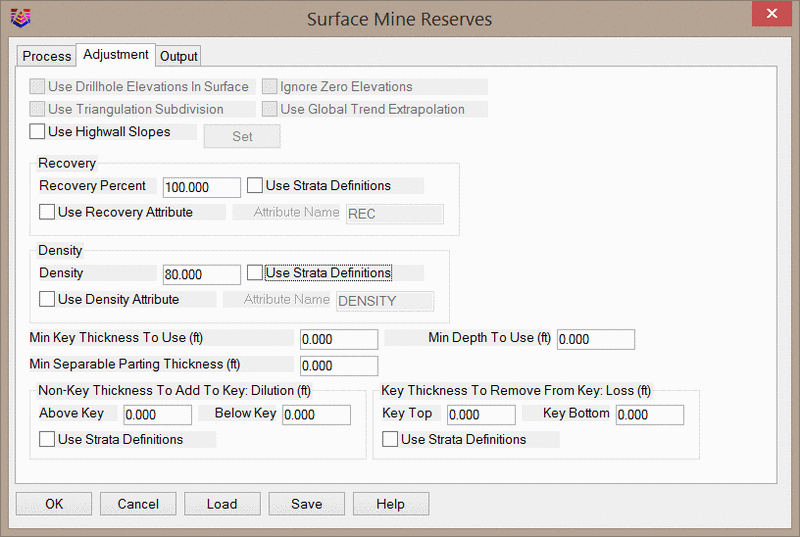
Adjustment Tab
Use Drillhole Elevations in Surface: When calculating the
reserves directly from drillholes, this option determines if the
drillhole collar elevations will be used to generate the
topographic surface.
Ignore Zero Elevations: When calculating reserves
directly from drillholes, this option will determine if entities at
zero elevation will be used to generate the topographic surface.
Generally, this option is useful in that it allows you to broadly
select entities in the drawing without manually filtering out zero
elevation entities.
Use Triangulation Subdivision: This option only applies
when using the Triangulation or Polynomial modeling methods to
calculate reserves directly from drillholes. When enabled, this
option will subdivide triangles to create smoother
surfaces.
Use Global Trend Extrapolation: This option only applies
when using the Triangulation or Polynomial modeling methods to
calculate reserves directly from drillholes. When enabled, this
option finds the average slope and direction of the interpolated
data and applies this slope to extrapolate to the full extents of
the grid.
Use Highwall Slopes: This option will apply highwall
slopes to the inclusion polylines to simulate a more realistically
shaped pit. This option is limited in that the inclusion polylines
selected for reserve calculation must represent the toe of the
highwall. This option will project highwalls upwards until it
reaches the topography. This option does not account for benches,
and so more complex calculations will need to be made using a
Surface History File generated from the Design Bench Pit
command.
Set (Slopes): This button will open the dialog shown
below, which controls the highwall slopes to use.

Highwall Layer: This field sets the layer to use for the
highwall linework. This linework will be drawn as a 3D polyline
where the highwall projection meets the surface.
Slope Type: This option controls if the highwall slope is
expressed as a percent or as a ratio.
Smooth Slope Transitions: This option will
gradually transition between slope angles as depth increases around
the pit. In the above example, the pit will have an overall slope
ratio of 1.0 where the cut depth is between 50 and 100', and a
slope ratio of 1.5 for cut depths greater than 100'. In areas where
the cut depth is exactly 100', this option will smoothly transition
from a slope ratio of 1.0 to 1.5 rather than abruptly changing the
slope angle.
Slope in Series: This option will use all slope angles
specified in the dialog. Using the above dialog as an example, the
cut angle from 0-50 feet (or meters) will always be a 0.7 ratio.
After this first 50 feet (or meters) of cut, the slope will be a
1.0 ratio for the next 50 feet (or meters). Any remaining cut will
use a 1.5 ratio.
Repeat Slopes: This option will repeat the slopes with
specified depths until the projection meets the surface topography.
In the above example, the program will repeat cut ratios of 0.7 and
1.0 until it reaches the surface. Since no cut depth has been
specified for the 1.5 cut ratio, this slope angle will not be used
with this option.
Recovery Percent: This value will set the overall
recovery percent for key strata. This is applied after adjustments
for non-key dilution and key loss. The volume of material that is
not recovered will be reported as non-key material.
Use Strata Definitions: This option will use the recovery
percent specified in the current Strata Definition file. This
allows you to set a recovery for each strata individually.
Use Recovery Attribute: This option will set the recovery
percent according to an attribute defined in the drillholes or in
the Geologic/Mining Model. This allows you to use a grid file to
set the recovery percent, thus allowing the recovery of each strata
to vary.
Attribute Name: This field sets the recovery attribute
name to search for in the drillholes or Geologic/Mining Model. This
attribute name must exactly match the attribute in the
drillholes/model, or else the recovery percent will not be
applied.
Density: This value sets the density to use for
all strata. Density is always expressed in lbs/ft^3 or
kg/m^3.
Use Strata Definitions: This option will use the density
specified in the current Strata Definition file. This allows you to
set a density for each strata individually.
Use Density Attribute: This option will set the density
according to an attribute in the drillholes or in the
Geologic/Mining Model. This allows you to use a grid file to set
the density, thus allowing for a varying density within each
individual strata.
Attribute Name: This field sets the attribute name to use
for density in the drillholes or Geologic/Mining Model. This
attribute name must exactly match the attribute in the
drillholes/model, or else the density will not be applied.
Min Key Thickness to Use: This value sets a minimum key
thickness for reporting. Any areas where the key strata is less
thick that this value, the strata will be reported as non-key
discard material.
Min Depth to Use: This value sets a minimum depth of
cover for key strata for reporting. Any areas of key strata that
have less than the specified thickness of cover will be reported as
non-key discard material. An example use of this option is
accounting for oxidized coal that is (or is close to)
outcropping.
Min Separable Parting Thickness: This value will be used
as a tolerance for calculating volume of non-key material between
key strata based on thickness. For example, if this value is set to
0.5, any non-key material sandwiched between key strata that is
less than 0.5 feet (or meters) thick will be reported as key
material. Areas where the non-key strata is greater than 0.5 thick
will not be affected.
Non-Key Thickness To Add To Key
(Dilution): Above Key/Below Key: These values set the amount
of non-key thickness above/below each key strata that will be mined
with the key strata. This diluted non-key material will not be
mixed with the key strata, but will instead be reported as another
key strata layer. The final report, however, can be formatted to
account for the dilution of strata qualities.
Use Strata Definitions: This option will use the Dilution
values set in the Strata Definition File. This allows you to set
the Dilution for each strata individually.
Key Thickness To Remove From
Key (Loss): Above Key/Below Key: These values specify the
amount of key thickness above/below the key strata that will be
subtracted from the key. This amount will be subtracted from the
key quantities and reported as non-key material.
Use Strata Definitions: This option will use the Loss
values set in the Strata Definition File. This allows you to set
the Loss for each strata individually.
Output Tab

Output Elevation Grids: This option will create grid
files for the bottom elevation of each strata. Each grid will need
to be named separately, and so it is recommended to instead use the
Strata Grids Autorun to make these grids quickly.
Output Thickness Grids: This option will create composite
grid files for the total key thickness, non-key thickness, and key
tonnage (expressed in tons/sq ft or tonnes/sq m). Each grid file
will need to be named separately. Note that when the option to
Store Results in Pits is used, these grids will be referenced in
the pit polylines. When this option is used, you will also be
prompted to Divide Bench by Thickness. This division will create
three more grid files that represent the divided thickness.
Output Volume Solids: This option will create solids of
the mined bench according to the pit names. These solids will be
automatically saved in a PIT_MODEL folder as .mdl files. This
PIT_MODEL folder will be automatically created in the current
project folder.
Report Format: This option controls the format of the
report.
The One Row per Strata option will report each strata layer on a
separate row. This default option is the most commonly used report
format.
The All Strata on Same Row option will report all strata layers on
a single row. This creates many extra columns for the report, but
allows for easier comparison of pit volumes.
The Group Key/Non-Key Pairs option will place overburden strata on
the same row as the key strata. This option searches for similar
naming in the strata names. For example, the strata COAL_KEY and
COAL_OB will be grouped together due to the similarity of the
strata names.
Output Spoil File: This option allows you to create a
Spoil Source File (.spo file) for use with the Spoil Placement
Timing command. This file includes the volume and centroid location
of waste material to be placed in spoil piles.
The Off option will not create a Spoil Source File.
The Non-Key Only will only include non-key strata in the Spoil
Source File.
The All Strata option will include all strata in the Spoil Source
File.
Strip Ratio Output: This option allows you to output
stripping ratio as contours or a grid file. Stripping ratio is
always expressed as volume of non-key material per weight of key
material (yd^3/ton or m^3/tonne)
The None option will not output the stripping ratio as contours
or a grid file. Note that when this option is used, the stripping
ratio will still be calculated in the final report.
The Draw Contours option will output contour lines of the stripping
ratio. This option will use settings similar to those used in the
Contour from Grid File command.
The Grid File option will create a grid file that represents the
stripping ratio.
Type of Strip Ratio Contours/Grid: This option controls
how the stripping ratio is expressed when it is output to contours
or a grid file
The Instantaneous option will calculate the stripping ratio for
each individual grid node. This stripping ratio will account for
all non-key and all key material within the calculation limits -
any non-key material existing below the last key strata will also
be used for the calculation of the stripping ratio. When the
reserves are divided into benches, the stripping ratio will be
reported by-bench.
The Accumulative option is intended for use in situations where
the key strata outcrops and is relatively flat. The below images
illustrate the way this form of stripping ratio is calculated based
on direction. The program will first determine the lowest
Instantaneous stripping ratio in the calculation area. The program
will then determine in which direction the stripping ratio
increases the least. If mining were to start in the area of lowest
stripping ratio and then move one grid node in the direction of
least increasing stripping ratio, the Accumulative stripping ratio
would be based on all key and non-key strata between the start
point and the next grid node location. In other words, imagine that
mining starts at the outcrop of the key material. As mining
progresses into the hillside, the accumulative stripping ratio is
the overall stripping ratio of all material mined up to the current
position.

Report Formatter and Miscellaneous Notes
The Report Formatter displays all information calculated with
this command, as shown below. For general information on using the
Report Formatter, see the corresponding of the help manual.

Here it is important to note that when a parent seam has been
configured to split into two child seams according to the strata
definition file, the program will automatically report the splits.
For example, if seam A splits into B and C, the program will report
tonnage for seam A where it exists as a parent as well as seams B
and C where they exist as child seams.
As an additional means of dividing reserves, Cut Sets defined by
the GIS Module > GIS Tools Pulldown Menu > Polygon Processor
command will be considered when the reserves are calculated. If a
Cut Set has been defined for wetland areas with a name of
"Wetlands", an additional reporting field will be available in the
report format called PP_Wetland. This will show the amount of
strata inside the wetland area. Any strata outside the wetland area
will be reported separately.
The report formatter will include two forms of stripping ratio:
"Strip Ratio" and "Strip Ratio Accumulative". The latter term
should not be confused with the Accumulative Stripping Raio for the
stripping ratio grid/contour output. Consider four strata layers:
A, B, C, and D where stratum A and C are non-key while stratum B
and D are key. When these four stratum are calculated on a single
bench, the report will include a "Strip Ratio" and 'Strip Ratio
Accumulative" for stratum B and D. Both attributes reported for
strata B report the stripping ratio as if only strata A and B were
mined. The "Strip Ratio" for strata D will report the stripping
ratio as if only strata C and D were mined. The "Strip Ratio
Accumulative" reported for strata D will report the stripping ratio
as if all strata above it were also mined (stratum A and B will be
included). The below image is an illustration of this
concept.

Miscellaneous note on block models: When the program detects a
Geologic Model containing one or more Block Models (.blk files),
the thickness of the strata containing the block model will be
compared to the thickness of the block model itself. Recall that
each strata in a Geologic Model is defined by the difference
between two elevation grids (or a thickness grid). Also, a block
model will be defined with upper and lower limits (also two
elevation grids). If the strata thickness is greater than the block
model thickness, the program will extend the block model thickness
an extra half-block height on the top and bottom of the
model.
Carlson block models will always have top/bottom layers of
blocks with half the height of other blocks (for more information
on this, see the section of the help manual corresponding to the
Make
Block Model command). To account for the full block size,
surface mine reserves applies the above logic. The idea is that
whenever the true strata thickness is thicker than the block model
thickness, the extra top/bottom block height needs to be accounted
for.
Prompts
Surface Mine Reserves dialog
Select surface entities and at least 3 drillholes. (Unless
using a Geologic Model File PRE.)
Select objects: select the drillhole symbols and surface
entities. Surface entities can include points, lines, and
polylines.
Select the Inclusion perimeter polylines and ENTER for none:
Select objects: select the polylines or named pit
polylines. The area within these polylines will be included in
the calculations. They must be closed polylines.
Select the Exclusion perimeter polylines and ENTER for none:
Select objects: select the polylines. The area within
these polylines will be excluded from the calculations. They must
be closed polylines.
Make Grid File Set grid resolution
Triangulating points ... 49
Pass> 6 NULL Z values left> 0
Processing cell 2500 ...
Finished strata Y2
The above four steps are repeated for each strata.
Report Formatter
Pulldown Menu Location: Geology Module > StrataCalc
and Surface Mining Module > Reserves/Timing
Keyboard Command: mtntop