- If you get the Start Page, pick New Drawing.
- If you get the Startup Wizard dialog box, click New.
- If you are taken directly into CAD, click the File -- New command.
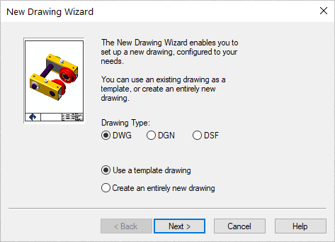
- Choose the DWG document type and the desire to base the
document on a Drawing Template as illustrated
below and then click Next >:
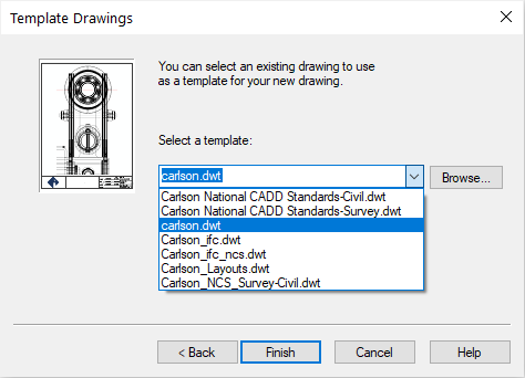
- Choose the carlson.dwt as illustrated below
(or surv.dwt if carlson.dwt is not available) and click
Finish:
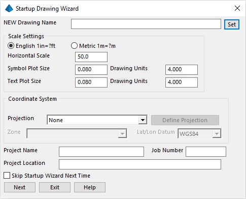
- We can now begin the more pertinent settings for the project to
come based on some preliminary settings that should be similar to
the default scenario shown below:
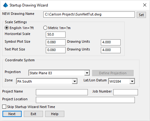
- Click Set at the top of the
dialog box, and enter in a NEW Drawing Name called
SurvNetTut. Verify that the other settings match
the settings shown below, and click Next:
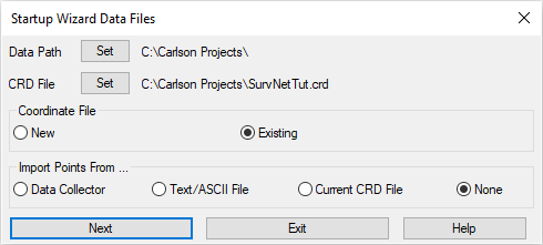
- You will see the Startup Wizard Data Files dialog to
set/confirm where to store data and indicate an information source
for points/coordinates. Set/match the values as shown below and
click Exit:
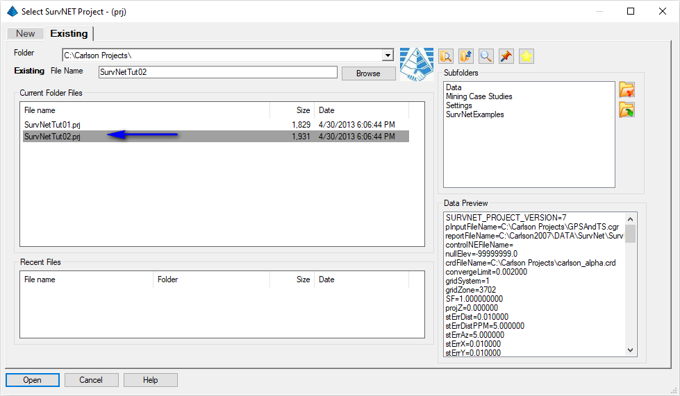
This, in turn opens the following dialog box:
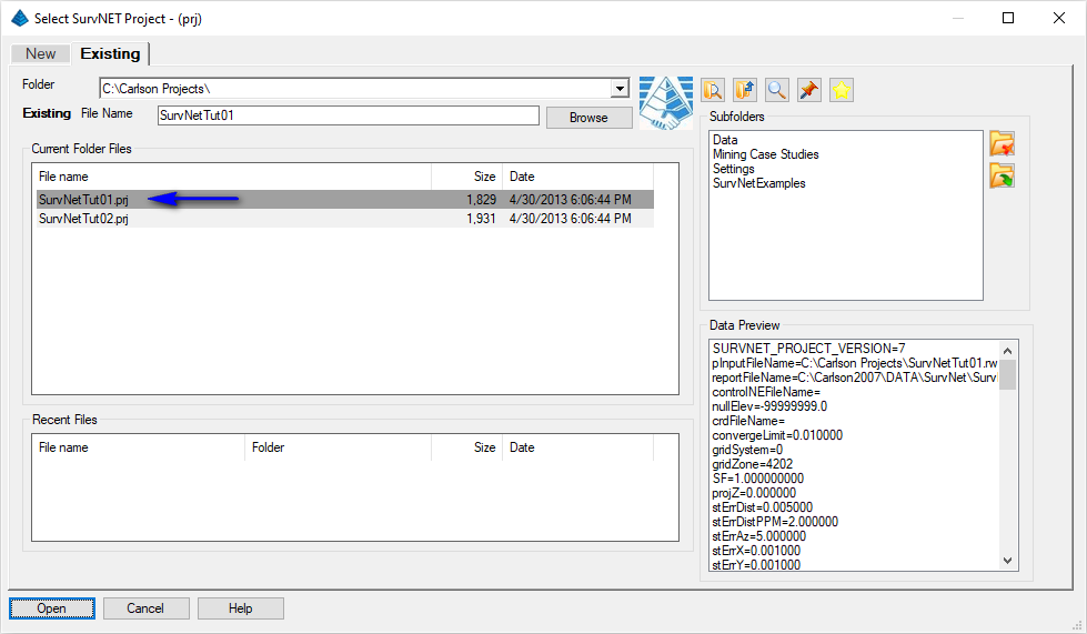
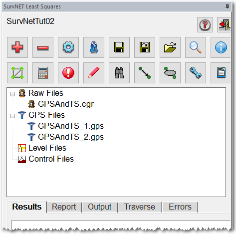
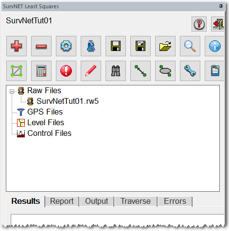
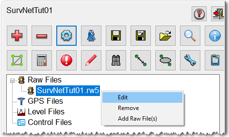
Select the SurvNetTut01.prj project and click Open. This will open the default SurvNET project-tree docked dialog box interface as shown below where we will process the contents of the SurvNetTut01.rw5 "raw" file:
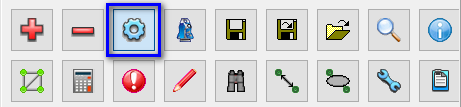
to display the dialog box below:
NOTE: In this dialog, the different settings required for the Least Squares reduction are available in the different tabs of the dialog box. When all of the settings are set as desired, click OK to save the changes.
-
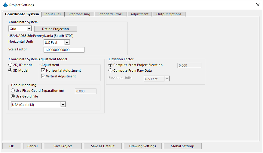
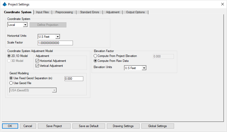
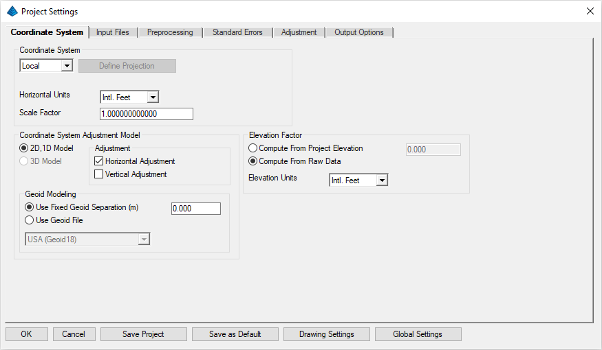
Settings - Coordinate System: For the purpose of this tutorial,
the Coordinate System settings tab should look as
follows before proceeding to the next step. To use an assumed
coordinate system, the Local Coordinate
System needs to be selected, and the
2D,1D Adjustment Model must be chosen. When using a local
coordinate system, the distance units are not important other than
for display purposes in the report. Computing elevation factors and
performing Geoid modeling is not applicable to assumed
datums. Notice that in this example we are not performing a
vertical adjustment (make this and other changes as
applicable):
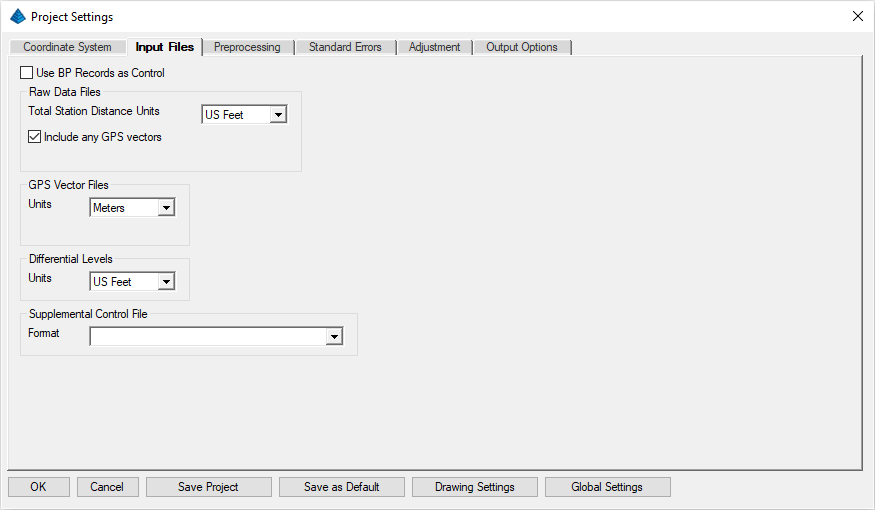
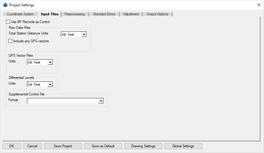
- Activate the
Input Files tab. The Input Files settings is where you
establish pertinent values for how the files are treated. SurvNET
allows you to have multiple raw files in a single project. The
ability for multiple raw files allows flexibility in collecting the
data and processing large projects. It is typically easier in a
large project to analyze and edit subsets of the total project,
before combining all the data for a final adjustment. Notice that
since we are working in a Local coordinate system and
using the 2D,1D Adjustment Model, GPS vectors cannot be
incorporated into this project. Make any necessary changes to match
the values shown below:
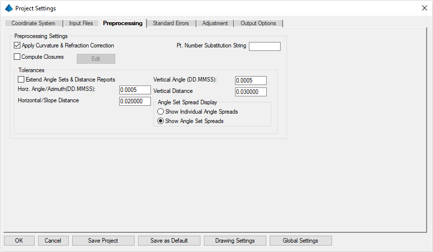
- Activate the
Preprocessing tab to review the Preprocessing settings.
Preprocessing consists of reducing and averaging all the multiple
measurements, applying curvature and refraction correction,
reducing the measurements to grid if appropriate, and computing
unadjusted traverse closures if appropriate. Much of the data
validation is performed during the preprocessing step. For the
purpose of this tutorial, the Preprocessing
settings should look as follows before proceeding to the next
step:

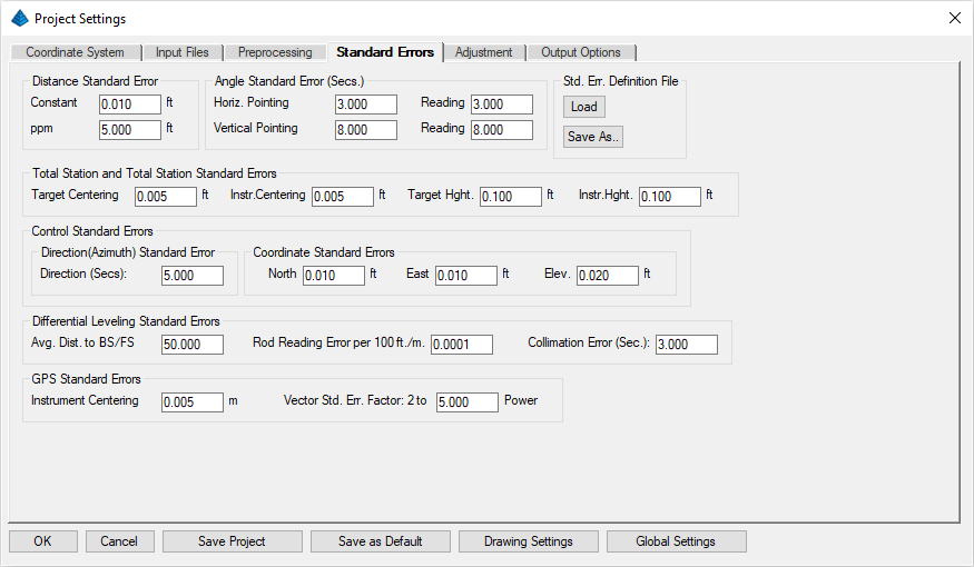
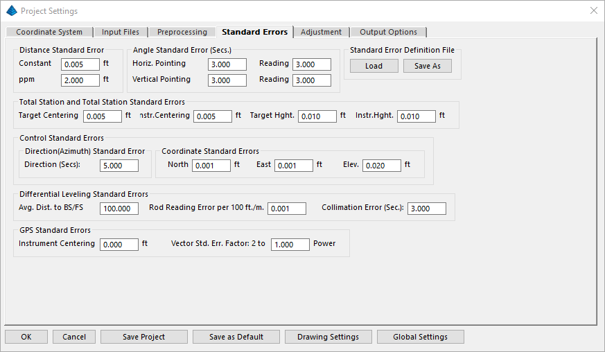
- Activate the
Standard Errors tab to review the Standard Errors settings.
Standard Errors are an estimate of the different errors you would
expect to obtain based on the type equipment and field procedures
you used to collect the raw data. For example, if you are using a 5
second theodolite, you could expect the angles to be measured
within +/- 5 seconds (Reading error). The Standard
Errors settings should look as follows before proceeding
to the next step:
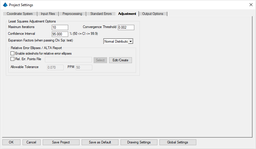
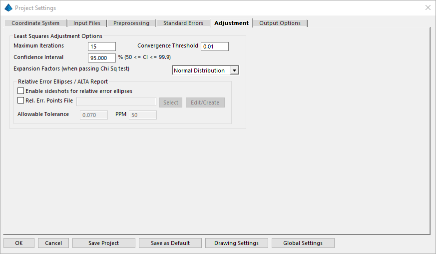
- Activate the
Adjustment tab to review the Adjustment settings. The
Adjustment settings affect how the actual Least Squares portion of
the processing is performed. Additionally, from the screen the user
can set whether ALTA reporting is performed. The Adjustment
settings should look as follows before proceeding to the next
step:
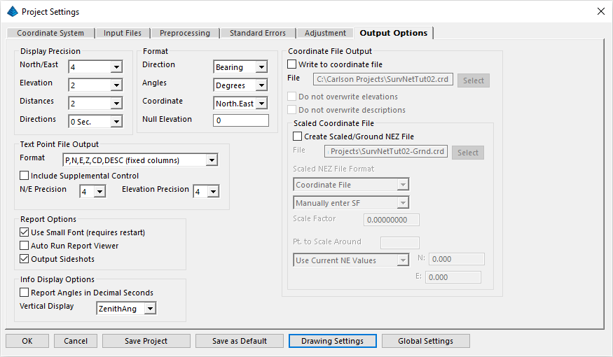
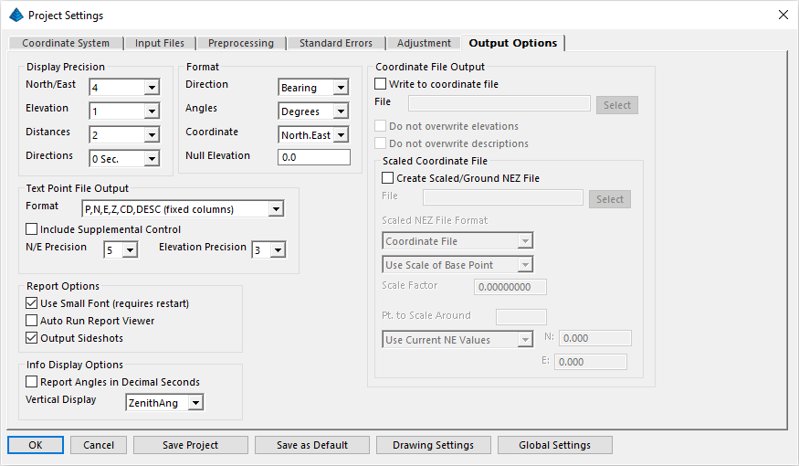
- Activate the
Output Options tab to review the Output Options settings. These
settings apply only to the output of data to the report files.
These settings do not affect computational precision. For the
purpose of this tutorial, the Output Options
settings should look as follows before proceeding to the next step.
Press OK to return to the main SurvNET
screen.
Review the following Standard Errors and Control Points discussion before exiting the Raw File editor:
- The default Standard Errors for points are
defined in the Standard Errors tab of the
Settings command as discussed earlier. There are
times when the default values may need to be overridden. For
example, the control may be from GPS and the user has differing
Standard Errors for various GPS points. Or maybe some of the
control points were collected with RTK methods, and other GPS
points collected with more accurate static GPS methods. Standard
Error for individual points can be inserted into the raw data file
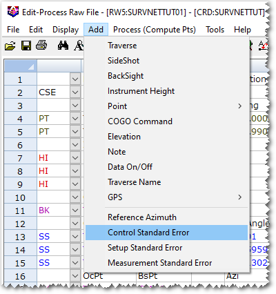
that will supersede the otherwise default values. The following is
the menu option used to insert Control Standard Errors
into the raw file:
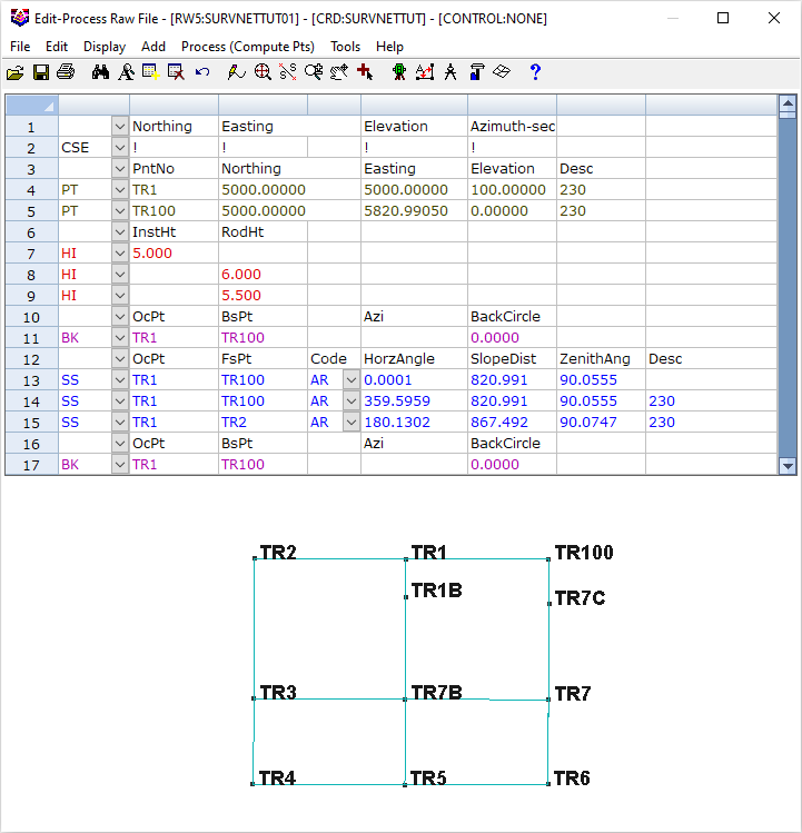
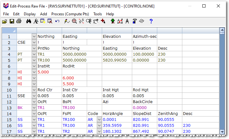
Notice in the above raw data file that points TR1 and TR100 are the Control Points for this project. Also, notice there is a Standard Error record (CSE) preceding the control points. - The CSE record has the Exclamation (!) character in the N,E,& Z field. The '!' character designates that all following control points will be "fixed." Points that are fixed will not be adjusted during the adjustment. Placing a very small Standard Error on a control point is almost equivalent to fixing the point. Points can also be designated to be floating points by using the Number sign (#) character. The only practical use of creating a floating point is if SurvNET cannot compute preliminary coordinates because no control point is occupied. The surveyor can compute a preliminary value for one of the occupied points, and insert that point as a floating point. The floating point will be adjusted, and no weight will be given to the floating coordinate values.
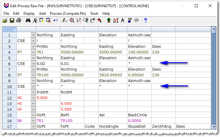
- Standard Error records affect all the records that follow the
Standard Error record. To revert the Standard Errors back to the
default values, a CSE record can be inserted containing the Asterix
(*) character. In the following example (shown for
illustrative purposes), point TR1 has been
designated as a fixed point. TR100 has a Northing
Standard Error of 0.02 and an Easting Standard
Error of 0.01. Additionally, the Elevation for
point TR100 would not change. Following the
TR100 point record is a CSE record containing the
'*' character in all fields. So, if there were any control points
further down in the raw data file, they would use the default
Standard Errors as set in the Settings dialog
box.
- There may be times when non-Control Standard Errors need to be overridden for certain measurements. For example, if fixed tripods were used for backsights and foresights for part of the traverse, and hand-held rods were used for another portion of the traverse, it would be appropriate to have differing Rod Ctr Standard Errors for the different sections of the raw data.
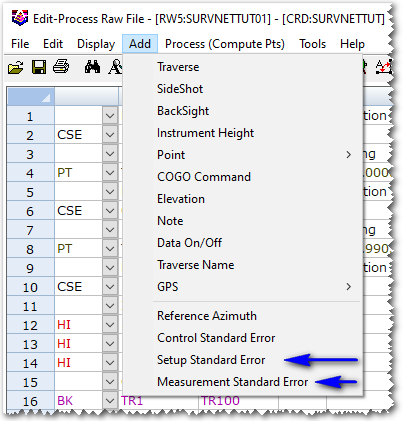
- Standard Errors for angles and distances can also be inserted
into the raw data file using Setup Standard Error
and Measurement Standard Error commands as
indicated below:
The Standard Errors set by these inserted records override the default Standard Errors. In the following example, a Setup Standard Error (SSE) record has been inserted in record 11. The SSE record affects all setup data that follow until another SSE record is inserted. In the following example, the Foresight Rod Centering error is set to 0.005, the Total Station Centering error is set to 0.005, the Total Station Measure-up error is set to 0.005 and the Foresight Measure-up error is set to 0.005:
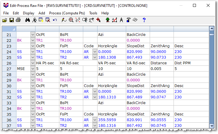
- The following is another example where it would be appropriate
to insert a Measurement Standard Error (MSE)
record into the raw data. If two different total stations with
different accuracy specifications were used to collect the data, it
would be appropriate to have different standard errors for the
different sections of the raw file, depending on which total
station was used to collect the data. In the following example, a
MSE record has been inserted for record 27. The
Horizontal Pointing and Reading error has been changed to 5
seconds, and the Vertical Pointing and Reading error has been
changed to 10 seconds. The inserted MSE record will affect
all following raw data until another MSE is
inserted:
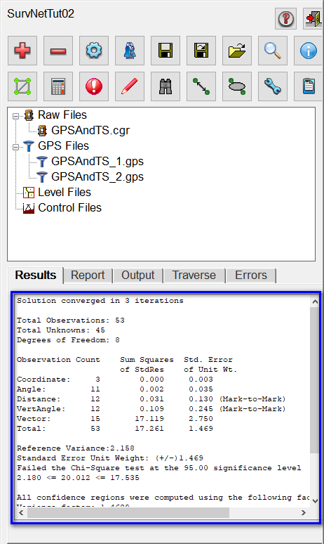
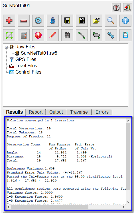
The least squares adjustment is performed, and the results from the adjustment are displayed. If the solution converged correctly, the report should look similar to the following window:
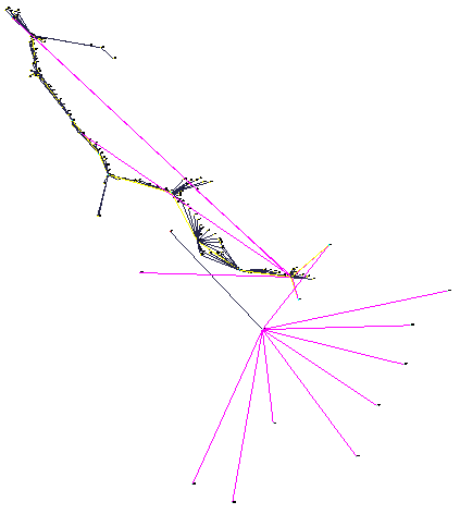
If there were errors or the solution did not converge, an error message dialog will be generated. If there are errors, you will need to return to the Raw File Editor to review and edit the raw data. Since the tutorial example should have converged, we will next review the various forms of output, including graphical representations of the adjusted network which can be:
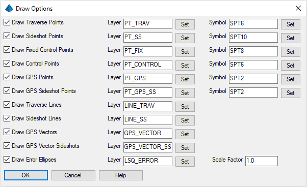
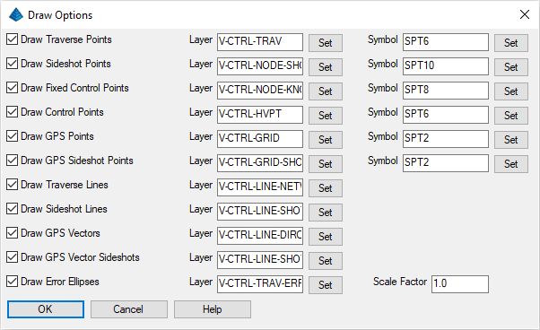
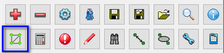
- Drawn into CAD through the Draw (Pencil) button, and/or
- Temporarily previewed through the Quick View (Binoculars) button.
- The .rpt file (Main Report), which is the primary Least Squares report file summarizing the data and the results from the adjustment,
- The .out file (Output Report), which contains a listing of the final coordinates,
- The .err file (Error Report), which contains any errors or warnings that were generated during processing,
- The .res file (Results Report), which contains statistical data that was generated during processing.
- Main Report button to display a
report similar to that shown below:
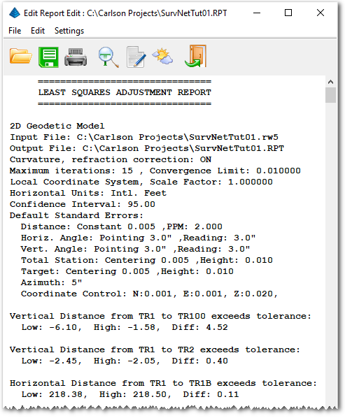
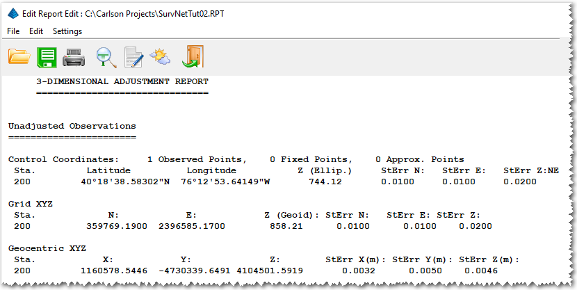
The excerpt from the report above shows the header information and the preprocessing results. The header information consists of (among other things), the input and output file names, the coordinate system, the curvature/refraction setting, maximum iterations, and distance units. During the preprocessing process, multiple angles are reduced to a single angle and multiple slope distances, vertical angles, HI's, and rod heights are reduced to a single horizontal distance and vertical difference. During this process the horizontal angle, horizontal distance and vertical difference spreads are computed. If the spreads exceed the tolerance settings from the Settings dialog box, then a warning message is displayed showing the high and low measurement and the difference between the high and low measurement. Continue to explore this report...- In the Unadjusted Observations
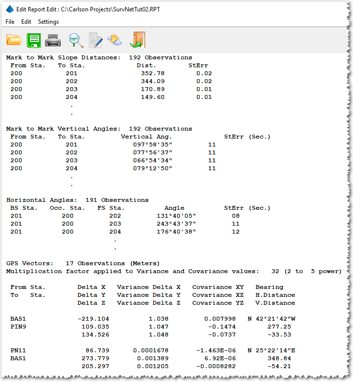
section will be data similar to that shown below:
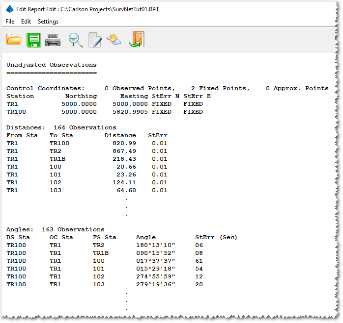
The excerpt from the Unadjusted Observations report above consists of some combination of control X, and Y, horizontal distances, horizontal angles, and azimuth measurements. These measurements consist of a single averaged measurement. For example, if multiple distances were collected between two points during data collection, only the single averaged measurement is used in the Least Squares adjustment. Also, Standard Errors for the measurements are displayed in this section of the report. The Standard Errors are computed from the Standard Error settings in the Settings dialog box using error propagation formulas. The Standard Error of an angle that was measured several times would typically be lower than an angle that was measured only once.
NOTE: If the data had been adjusted into NAD 83 coordinates both the ground distances and the grid distances would be displayed. The grid, elevation, and combined factor would also be displayed in this section of the report. Continuing into the report: - In the Adjusted Observations section
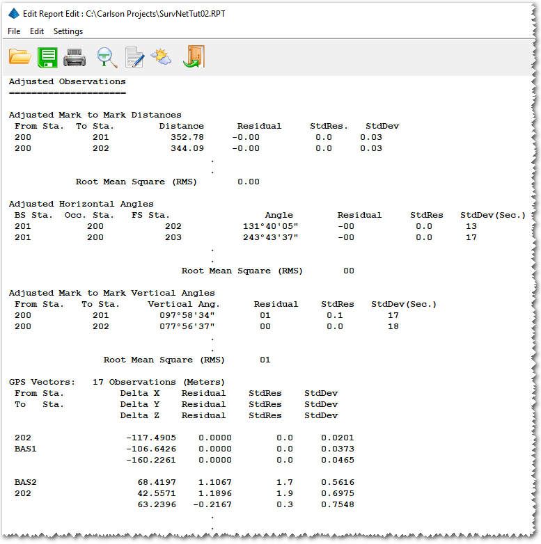
will be data similar to that shown below:
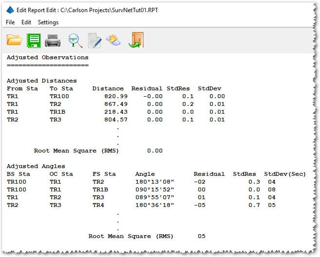
The excerpt from the Adjusted Observations report above shows the final adjusted measurements. This section is one of the most important sections to review when analyzing the results of the adjustment. In addition to the adjusted measurement, the Residual is displayed. The Residual is the amount of adjustment applied to the measurement and is computed by subtracting the unadjusted measurement from the adjusted measurement.
The Standard Deviation of the measurement is also displayed. Ideally, the computed Standard Deviation and Residual and the Standard Error displayed in the unadjusted measurement would all be of similar magnitude. The Standard Residual is a measure of the similarity of the Residual to the a-priori Standard Error. The Standard Residual is the measurements Residual divided by the Standard Error displayed in the unadjusted measurement section. A Standard Residual greater than 2 is marked with an "*". A high Standard Residual may be an indication of a blunder. If there are consistently a lot of high Standard Residuals it may indicate that the original Standard Errors set in the Settings dialog box were not realistic. - If the Enable sideshots for relative
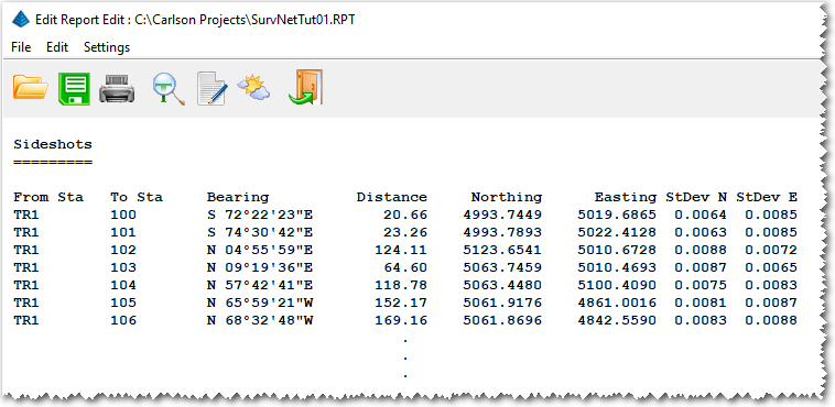
error ellipses option is not set in the Adjustment section of the Settings,
sideshots are computed separately after the adjustment is
completed.
If the project had valid elevation benchmarks and measured HI's and rod heights the project could have been defined to adjust elevations. When using the 2D/1D Least Squares model, the horizontal and the vertical adjustments are separate Least Squares adjustment processes. As long as there are redundant vertical measurements, the vertical component of the network can also be reduced and adjusted using Least Squares. In the vertical adjustment, benchmarks are held fixed. Click the Exit (Doorway) button to dismiss this report.
- In the Unadjusted Observations
section will be data similar to that shown below:
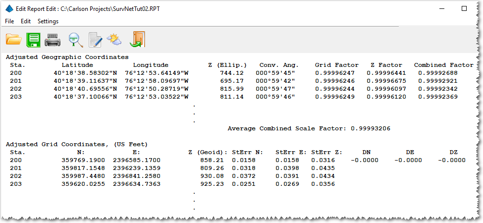
- Output Report button to display a
report similar to that shown below:
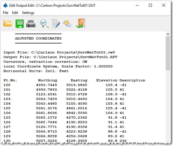
This section of the report shows the final adjusted coordinates. Click the Exit (Doorway) button to dismiss this report. - Error Report button to display a
report similar to that shown below:
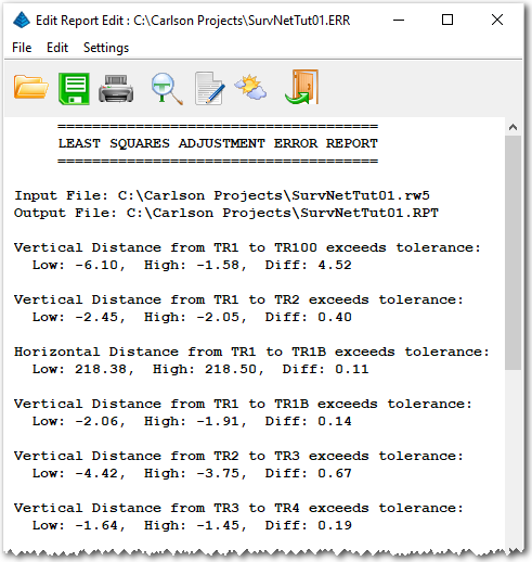
This section of the report is one of the simplest and effective tools in finding blunders. Time spent learning how this function works will be well spent. If the project is not converging due to an unknown blunder in the raw data, this tool is one of the most effective tools in finding the blunder. Many blunders are due to point numbering errors during data collections, and the K-matrix analysis and Point Proximity search are great tools for finding these types of blunders. Click the Exit (Doorway) button to dismiss this report. - Results Report button to display
a report similar to that shown below:
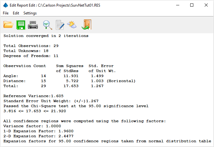
This report displays some statistical measures of the adjustment including the number of iterations needed for the solution to converge, the degrees of freedom of the network, the reference variance, the standard error of unit weight, and the results of a Chi-square test.
The degree of freedom is an indication of how many redundant measurements are in the survey. Degree of freedom is defined as the number of measurements in excess of the number of measurements necessary to solve the network.
The standard error of unit weight relates to the overall adjustment and not to an individual measurement. A value of one indicates that the results of the adjustment are consistent with the prior standard errors. The reference variance is the standard error of unit weight squared.
The Chi-square test is a test of the "goodness" of fit of the adjustment. It is not an absolute test of the accuracy of the survey. The a-priori standard errors which are defined in the project settings dialog box or with the SE record in the raw data file are used to determine the weights of the measurements. These standard errors can also be looked at as an estimate of how accurately the measurements were made. The Chi-square test merely tests whether the results of the adjusted measurements are consistent with the a-priori standard errors. Notice that if you change the project Standard Errors and then reprocess the survey, the results of the Chi-square test change, even though the measurements themselves did not change.
In our example, the Chi-square test passed at the 95% significance level. Had our example failed the Chi-square test on the low end (e.g. a value < 3.816), indications would be that our data is actually better than expected compared to our a-priori standard errors. If we were to increase the Pointing and Reading Standard Error in the Settings menu by 10-20 seconds, we would probably fail the Chi-square. Also notice that if you change the Standard Errors by only 5-10 seconds and reprocess the data the final coordinates will not change significantly.
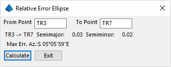 Enter
TR3 and TR7 in the From
Pt. and To Pt. fields, respectively, and
click the Calculate button. At the 95% confidence
level there should only be around 0.03 feet of error between points
TR3 and TR7. If you need to compute Relative Error Ellipses for
sideshots, make sure the Enable Sideshots for Error
Ellipse toggle is set in the Adjustment tab of the Settings dialog box. Click the
Exit button to dismiss the Relative Error
Ellipse dialog box. Click the Exit (Doorway)
button to dismiss the SurvNET docked dialog box.
Enter
TR3 and TR7 in the From
Pt. and To Pt. fields, respectively, and
click the Calculate button. At the 95% confidence
level there should only be around 0.03 feet of error between points
TR3 and TR7. If you need to compute Relative Error Ellipses for
sideshots, make sure the Enable Sideshots for Error
Ellipse toggle is set in the Adjustment tab of the Settings dialog box. Click the
Exit button to dismiss the Relative Error
Ellipse dialog box. Click the Exit (Doorway)
button to dismiss the SurvNET docked dialog box.