
Geologic Model Elevation Model

Geologic Model Thickness Model
Surface and Underground Reserves are the key routines for developing reserve estimates and qualities and for setting up equipment-based mine scheduling. Along with the Fence Diagram routine, Surface or Underground Reserves will calculate strata elevations and qualities using Geologic Model grids. These grids represent the "mine model". Here we will study how to make the grids strategically to build in well-defined subcrops, outcrops, splits, correct strata thicknesses, and qualities.
What is the "Geologic Model"
File?
The Geologic Model File can either be an Elevation model or a
Thickness model. The elevation model consists of a grid model of
the surface topography as the first and primary grid. Below the
surface grid is the bottom elevation grid for each strata to be
modeled, ordered top to bottom in the Geologic Model grids dialog
box. Any number of quality attribute grids (covering such items as
sulfur, ash, moisture, etc.) can be associated with the bottom
elevation grid of a particular strata, though they are not
required. If a strata is called C1, for example, the C1 name is
associated with its bottom elevation grid file, and any attribute
grid files should refer to the same Strata name. A Thickness
Geologic Model just contains thickness grids (no elevation grids).
There is no surface topo grid file defined in a thickness model.
Below are typical examples of both types of Geologic Model
files.
Geologic Model Elevation Model
Geologic Model Thickness Model
When naming attributes such as Ash, BTU and Moisture, be sure to attach the attributes to a strata (in this case C1 and C2) which must match the exact spelling of the strata name containing the associated base elevation or thickness grid. These names are not case sensitive, and are converted to upper case automatically.
Grid Cell Dimensions
Drillholes at many mines are often drilled at a spacing of 500 feet
or more, making small cell size unnecessary when modeling geologic
aspects, especially quality attributes. As a rule of thumb, cell
size should be 1/4 the average drillhole spacing between drillholes
for most accurate modeling. With some minerals and ores such as
quality controlled limestone and clay, drillholes are drilled as
close as 50 feet apart. This would suggest the need for a 12.5-foot
cell size or less. Surface topography, however, often demand the
tightest cell size, because the topography can include steep
cliffs, high stream banks and other abruptly changing features,
that can be lost or smoothed if cell size is on the order of
100' to 200' spacing. Below are two examples of surfaces. The first
surface has gently sloping terrain and widely-spaced contours. This
has been gridded at 100'x100', as there are no sharp features that
need to be captured in the grid file. The second set of images
shows an open pit with benches, spoil and roads. To accurately
capture all of this detail, a grid size of 10'x10' is more
appropriate. It makes a much larger file, but does not over-smooth
the surface, as a larger grid cell size would do. There is no
limit, but try to keep the number of total cells in a grid file
less than one million total cells. It will run much faster if each
grid file is less than one half of a million grid cells.


Cell Positions and Dimensions Should Match
Some routines in Carlson require that the grid position and cell
size should be identical for all grid files in a Geologic Model
grid model set (Design Bench Pit is an example). To ensure that
grids match position and dimension, make the first grid file, then
make all additional grid files based on the position of the first
grid file. To do this, you select option "F" when prompted: Use
position from another file or pick grid position
(<Pick>/File)? There are Grid File Utilities to modify grids,
such as Change Position, Change Resolution and Match
Dimensions.
In Surface and Underground Reserves calculated from a Geologic
Model, the grids do not need to match. It is common to have a
surface topo grid file with a small cell size, such as 10x10. Then
the structure grids for elevation or thickness could have a medium
cell size, such as 50x50. Finally, quality attribute grids can have
an even larger cell size, such as 200x200. This could be due to the
fact that not every drillhole has quality sampled, so the spacing
of quality holes is much greater than structure data holes, not
needing a tight resolution. Here it is important to note that when
volumes are calculated, the elevation and quality grids will be
temporarily resized to match the topography (note that the grids
themselves will not be permanently modified).
Cell Dimensions Versus Number of Cells
Carlson defaults to 50x50 "number of cells" when first installed,
meaning that in any grid window position, there will be 50 cells in
the X-direction and 50 cells in the Y-direction, unless altered by
the user. If the window is longer in the x-direction, then the
cells will be longer in their X-dimension than in their
Y-dimension, creating rectangular shaped grid cells. By contrast,
the user can specify the cell dimension when making grids, leading
to a variable number of cell, depending on the size of the grid
window. It should be noted that the default itself can be set by
the user. This is done by selecting Carlson Configure under the
Settings Pulldown Menu > Surface Settings, which provides the
following dialog. Note that at the bottom of the dialog there is
the option to set the number of cells or the dimension of the cells
to any desired value.

Make Top of Strata Grids by Adding Thickness Grids to
Bottom of Strata Grids
The elevation Geologic Model File is based on having grid files for
the bottom and top of all key strata. If you have only the surface
grid, and the bottom and top elevation of each Key strata, you are
set up for most reserve and scheduling work. Of course, quality
grids can be added, and NonKey elevation grids such as base of
unconsolidated overburden are valuable. But the point here is that
you want bottom and top of Key grids for each seam under
consideration. These grids should in most cases be made by making a
thickness grid for the strata and adding thickness to base
elevation to obtain top of strata grids. There are two settings
that should be monitored when doing this type of modeling. Under
Settings > Carlson Configure > Mining Settings, be sure that
pinch-out is on for modeling thickness. If not, then the seam will
never pinch out in cases of zero thickness holes. When modeling
elevation grids, it is often helpful that pinchout turned off,
because when it pinches out a seam, it sometimes brings that
elevation up to the next seam above, to pinch it out. If pinch out
is off, it will keep the elevation grid down where it should be,
had the seam been there. Add the two grids together to get the
roof. Where the seam had zero thickness, the roof will be the same
as the floor, and down and the correct elevation. The following
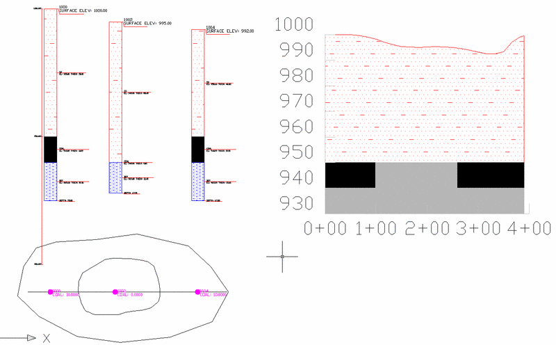
example shows this concept, where the middle seam is pinching out
in the middle. The middle hole has a zero value for coal thickness.
This will bring the coal up to that hole, then pinch it at the
hole.

This next example is created from the example where the Coal seam does not exist in the middle hole, not even a zero. This method will pinch the coal 1/2 way between the holes, based on the Pinchout Settings under Carlson Configure > Mining Settings. Most of the time, this is your best guess.

Using slightly different settings, this next Fence Diagram can be obtained.
Two Strata Limit Polylines were drawn around the drillholes, representing crop lines. The interior line is an exclusion limit line. The outer line is an inclusion limit line. The grids were remade, the bottom elevation and the thickness were added together to get the new roof, and here is the result. The seam carries its full thickness to the cropping limit lines, no pinching is taking place.
Grid File Utilities
The Grid File Utilities can be accessed from within the Geology
Module by entering GFU in the command line, or under the Grids
Pulldown Menu > Grid File Utilities. It is also located in the
Surface Pulldown Menu of the Civil Module. After starting the
command, you must first choose Select Grid(s) to load a grid file.
Within GFU, you can click an option to be prompted for
Inclusion/Exclusion perimeter polylines. The grid manipulation will
only occur inside or outside these perimeters. The commands BPoly
and Shrinkwrap under the Draw Pulldown Menu are useful tools to
generate these perimeters.

Adding One Grid to Another
In order to add grids, select Grid File Utilities (GFU) to bring
up the dialog box shown above. Choose Select Grids and load the
base elevation of the coal seam, COAL_ELV.GRD. The next step is to
select Math Functions > ADD GRID which asks for the grid file to
load (COAL THK.GRD). At this point you would choose "SaveAs" and
save the result as "COAL TOP.GRD". If this modeling effort is a
one-time process, there is no need to save a macro that allows for
automatic re-running of the grid addition. However, if the
thickness grid or base of coal grid might change due to the
addition of more drillholes (or the editing of existing
drillholes), then macros can be time-saving devices. To make a
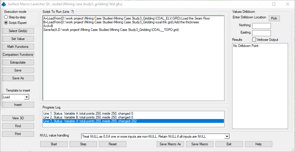
macro for our example, you would get to the dialog above by
entering GFU as before and clicking the Macro Editor button.
First, create a new GFU file for future Auto-Run. Then Choose the
Select Grid button. The upper right button in GFU Load Grid Options
allow user to choose grid file.

The Grid Variable "A" at the top represents the grid file to be
loaded. So A is COAL_ELV.GRD (the base of COAL grid). Repeat
loading the second grid and use Grid Variable B for the COAL
THK.GRD thickness grid. Next click Save As, same as above. Now
select Start to run the macro. Note that you may manually modify
the text in the macro as needed. Comments can be added by typing
";" at the beginning of the comment. For example, the below line
will load a grid file, but will recognize the end of the line as a
comment rather than part of the actual macro.
A=LoadFrom(D:\work project\Mining Case Studies\Mining Case
Study3_Gridding\COAL_ELV.GRD);Load the Seam Floor
The Need to Extrapolate
Some modeling methods (Inverse Distance, Kriging, Linear Least
Squares, Nearest Neighbor, and ABOS) will automatically extrapolate
the grid, filling in values entirely within the limits of the grid
location. If the modeling is done by Triangulation or Polynomial,
the grid values will only exist within the area of the data points
- everything beyond the data points will be empty. Thus the area of
modeling by Triangulation or Polynomial will always be less than
the area of modeling by any other method. This may create a problem
in Grid File Utilities where grid addition is involved. Two things
can happen. Number one, the program may complete the addition, but
in reality grid values have not changed where the base grid file
contained null values. Number two, the program may report "Grid
files do not match" and refuse to do the grid math operation. To
remedy this, choose "Extrapolate" within Grid File Utilities,
select the default method, and extrapolate all grids prior to doing
grid math. The extrapolate command itself can become part of the
macro if record or append is selected. Other routines have the
option to extrapolate, such as Grid Inspector, where there is a
check-box to Extrapolate Grids. The Reserve commands will always
extrapolate the grids upon loading, so it is generally preferred to
make sure they are extrapolated to start with. There are two
options at the bottom of the Define Geologic Model dialog to
extrapolate the grids. One method will extrapolate the elevation
out, the other will merge with the next upper seam, pinching the
thickness to zero.
Reserves from Geologic Model
Grids
It is always preferable to compute volumes from Geologic Model
files using the Surface or Underground Mine Reserves. All the care
and control that went into making the grid files is then reflected
in the improved accuracy and legitimacy of the result. The Geologic
Model can contain quality attribute grids, and even a Block Model
for detailed quality tracking and breakdown. The alternative is to
select drillholes directly from the screen (on-the-fly), which
builds in uncertainty as to the nature of the modeling.
Choosing a Method of Gridding
Every user is confronted with the issue of what gridding algorithm
to choose. Here there is no substitute for experience and
verification in the field. We at Carlson Software have noticed that
many qualities such as sulfur or calcium are modeled most often by
Inverse Distance. Base elevation, in general, appears to be
amenable to the logic of Triangulation or Polynomial, much like
surface topography, though even here Inverse Distance is
often used. Strata thickness, however, is again more localized and
is often best modeled by Inverse Distance or Least Squares.
Polynomial surface modeling utilizes Triangulation, so again lends
itself to broad, large area influences. When and how to use Kriging
is an art in itself. We have found the "power" form of Kriging to
model effectively in evenly distributed drillhole data. The
following diagram shows the same drillhole data set modeled with 12
different versions of the algorithms. Notice there are some large
differences, yet all have their benefits.

Calculate Residuals
This command guides the user to select a modeling method. The
concept is much like field checking. With field verification, you
would pick a location for testing, then measure coal thickness or
sulfur or base elevation and check the data against the model. If
it is close, your model is good. If the testing is repeated, you
can add up all the errors (the residuals) and make a determination
of the effectiveness of one model against another. But even without
field testing, you can take 25 drillholes and model with 24, then
check the error residual at the removed drillhole. You can then
repeat this "removal" process across all 25 drillholes, and verify
the average residual error and the standard deviation of the
residual error. This is exactly what the command Calculate
Residuals does.

Shown below, for example, is a
comparison all the modeling methods exported to Excel. This was
done with Auto-Run Residuals command.

In this example, ABOS has the lowest standard deviation and
absolute value residual average, making it a stronger candidate for
modeling this drillhole dataset. The command Calculate Residuals
will bring up a report that shows every drillhole and what the
residual was. It will also create a Histogram, showing the number
of residuals within certain ranges. This can be used to look for
extreme values and fliers. However, it important to note that even
though a gridding method may have the most favorable residual
average, the contours and cross sections for that method should
still be analyzed for accuracy.

Modeling Options
It is important to set the strata modeling options that are in
Settings Carlson Configure command under Mining Settings. These
setting are used in modeling commands that process strata from
drillholes such as Make Strata Grid, Surface Mine and Underground
Mine Reserves, and Strata Isopach Maps, just to name a few.

The Inverse Distance and Least Squares settings control the data point search radius and the maximum samples which limits calculations to the nearest set of the specified number of data points. Inverse Distance and Least Squares can also be forced to use a minimum and/or maximum number of data points from each quadrant NE, SE, SW and NW. These inverse distance settings are used whenever modeling by inverse distance.
During strata correlation, the program matches strata with the same name between drillholes. When a strata name is missing in a drillhole, there are three possibilities. Either the program can skip that drillhole for modeling that strata, the strata pinched out, or the drillhole did not reach the strata and the strata position can be modeled by conformance. The method to use is determined by the Pinch Out and Conformance settings in this dialog.
If you turn off Pinch Out, then the program will skip a drillhole with a pinch out case for modeling that strata. Otherwise the missing strata will be given a negative thickness at the drillhole. The thickness is negative so that when modeled with the other positive thickness drillholes, the pinch out or zero thickness position will be somewhere midway between the missing and existing drillholes. The slide bar "Near Zero <-> Non-Zero" controls the amount of the negative thickness. The Near Zero setting will make a smaller negative value which moves the pinch out position closer to the missing strata drillhole. Likewise Non-Zero makes a larger negative value which moves the pinch out position closer to the drillhole with the strata.
For Conformance, turning off conformance will make the program skip a drillhole with a conformance case for modeling that strata. With conformance active, the missing strata position at the partial drillhole will be calculated by modeling the thickness between the missing strata and a marker strata that does exist in the drillhole. This thickness is modeled with inverse distance using drillholes where both strata exist. Then the thickness is added to the marker strata to locate the missing strata in the partial drillhole. Conformance can be set to Seam-Specific which allows only specified strata to be marker strata. Additionally, the specified marker strata will only conform with specified target strata. The marker and target strata names are set in Define Strata.
| Converted from CHM to HTML with chm2web Standard 2.85 (unicode) |