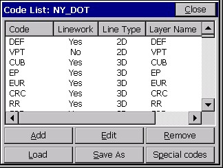
This command allows you to define feature code lists. You can create multiple feature code lists and each list can contain an unlimited number of codes. Each feature code consists of a short code, a longer description, a polyline toggle and a polyline type setting.  The initial dialog is shown here.

Add a Feature Code

• Add: To add a code to the list, select this button. The Add Code dialog will appear.

Select a Feature Code File

• Load: Select the Load button to select a file to open or edit. Choose an existing file or enter a new file name to create a new Feature Code List. Feature Code List files have a *.FCL file extension.

Edit an Existing Code

• Edit: If you wish to edit an existing code, double tap on the code or highlight it and tap Edit. It will appear in the Edit Code dialog.

Saving the Feature Code List

• Save As: Select the Save As button to save the file. Choose an existing file or enter a new file name to create a new feature code list.

Remove an Existing Code

• Remove: To remove a code from the list, highlight an existing code and press the Remove button. Carlson SurvCE will ask you to confirm deletion of the code.

The Add Code dialog is shown here. Below the dialog is a description list of the various options and buttons.

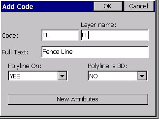
Code: Enter the name of the Feature Code. For example you might use EP for edge of pavement.

Full Text: Enter a description for the code. This is only for your information. It is not added to the point description.

Polyline ON: This setting determines whether points with this code are joined together with linework when the points are plotted.

Polyline is 3D: Choose whether the polyline should be 3D or 2D. If you choose YES, then each polyline vertex is located at the elevation of the point. If you choose NO, then the entire polyline is constructed on elevation 0 (zero), regardless of each point’s elevation. This setting is not applicable if Polyline ON is set to NO.

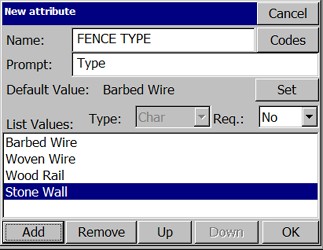
New Attributes: This option leads to “GIS” type attributing, where you can further describe the code (e.g.  fence) with additional attributes.  For example, one attribute might be Fence Type, and there may be 4 options, with a default option.  These can be set up, one time, by using the “Add” option within New Attributes, and then whenever a fence is chosen, the attributes can be selected from a list.  These attributes store in the raw file and most importantly, will output to an ESRI Shapefile (Map Screen, File Pulldown, Export SHP File).  You can even control the “prompt” and what the default attribute is (here “barbed wire”) and whether some attribute entry is required, or just optional.  With this setting, any shot to “FL” for fence will jump into the GIS attribute screen. The setup screen for attributes is shown in this figure.

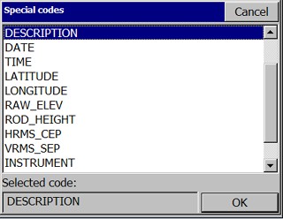
Fence type is a user-defined attribute.  But many attributes of the feature are “known” by Carlson SurvCE (eg. the current instrument being used, the date and time, etc.).  These types of “known” attributes appear in a list of selectable “Codes” -- selectable above, and shown in this figure below.

Now, when you are collecting the points with an “FL” code, and the program detects that you have shot a “point-only” feature, or if a line, that you have ended the line (eg. FL END), then you will be prompted for the attributes.

If there were several attributes associated with the fence (eg. height, condition, etc.), then Next and Previous buttons would be active.  If you had just shot three points along a fence line with GPS, the raw data file would appear, within COGO - Process Raw File - Edit Raw Data File.

You have the option not to save the attribute information, in which case it would not appear in the raw file or be convertible to shape files using the command Export SHP File found under File in the Map screen.

Special Code Suffixes

• Special Codes: In addition to the codes that you add to the Feature Code List, there are some predefined code suffixes that you may use to end lines or start curves.  For example, FL END could end the fence line, with “END” being a predefined “special code”.  You can substitute new codes for default codes, such that “..” can be substituted for “END” to end a line, which was the case above where the fence line ended with “FL..”.  The special code suffixes can also be entered as prefixes, as in PC EP (for start curve) rather than EP PC.  Special Codes should be separated from your actual feature codes by a space, however the alias of “..” can go right up against the feature code as in “FL..”. The special codes are described below.

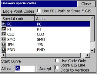
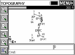
PC & PT: Used to specify the point of curvature (PC) and point of tangency (PT) of a curve. If you are taking shots on a curve, use PC to specify the beginning of the curve and PT to specify the end of the curve. The PC special code will activate a 3-point arc automatically, so use of the PT code in a 3-point arc is redundant and therefore it is not necessary.  However, if you are picking up a meandering stream or treeline, PT is useful to end the curving feature, and the program will “best fit” a curve through all the surveyed points between the PC and PT codes.

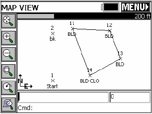
CLO: Use this code to close a figure. This tells the software to close from the last point coded as CLO back to the first point of the figure.

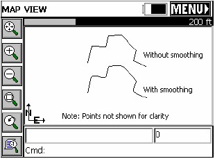
SMO: Use this code to smooth the line through all of the points. This code must occur on the first point of the line.

JPN: Use this code followed by a point ID to create a new line segment between the current point and the entered point ID.

END (or -7): Use this code to end the line.

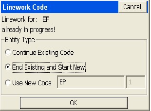
+7 (a.k.a. Begin):  Use this code for starting a line, which automatically ends any previous line with the same code already started.

Alias: All the special codes can be altered to suit your practices.  For example, if your crews start curves by the code CS (Curve Start) and end with CE (Curve End), these can be substituted for PC and PT as “aliases”.  Furthermore, the special codes can occur before the description or after the description (normal practice).  So whereas by default, curves might be coded EP, EP PC, EP, EP (no EP PT is needed, 3-point curves are default), coding could be EP, CS EP, EP, EP (through use of aliases).

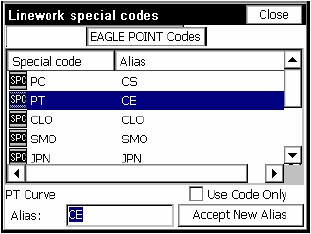
Accept: When you add an alias (like changing PT to CE for “curve end”, for example), press Accept to record the change.

Eagle Point Codes:  Here you can set special Field Code, End Line and Close Line coding to draw per Eagle Point conventions and set up normal processing of linework when downloaded to Eagle Point office software.

Use FCL path to store *.GIS :  The folder for the GIS data is normally hardcoded to one level deeper than the data directory.  By clicking this on, you can store the GIS files under a folder that has the same level as the FCL file.

Use Code Only:  With this clicked on, GIS attributing is ignored.  This can reduce the prompts on projects where no GIS attribute information is required.

Store GIS Line Data to Vertices:  For purposes of exporting to ESRI, you can store distinct GIS data to each vertice on a line or polyline, as opposed to associating one set of attributes to an entire line or polyline.

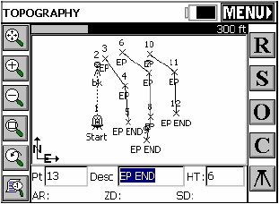
Note:  The main purpose of the flexible line coding is to create linework in the field that will be re-created in the office using office software.  The field linework is typically used for confirmation — if a curve is drawn, the field surveyors know it will create a curve when processed in the office, whether in Autodesk, Carlson or other types of office software.  But linework created in the field is stored as a DXF file and will draw in most CAD programs when copied from the CE device to the office PC.