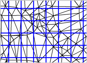
Make 3D Grid File

This command creates a grid (.GRD) file which serves as a surface model for use in many of the other Surface routines. The program internally makes a triangular network of the data points (if Triangulation is selected as the modeling method) and then interpolates the elevation values of a rectangular grid at the specified grid resolution. Data points can be either points, inserts, lines, or polylines. Lines and polylines are treated as breaklines in the triangulation.

Gridding as a means of modeling surface features is generally less favorable than triangulating as the surface is defined only at the intersection of the grid lines. This can lead to inaccuracies around local features such as ditches or curb lines, since the grid resolution must be small enough to adequately capture the changes in these local regions. Contrast this with Triangulated Networks which carry all this information at every point along the features. Gridding can, however, be useful for modeling large sites in general trends such as watershed analyses and large-scale volume computations.

Grid superimposed over triangulated features

The grid location is specified by first picking a lower left corner and then an upper right corner. The screen cannot be twisted when this is done because grids always run north-south and east-west.

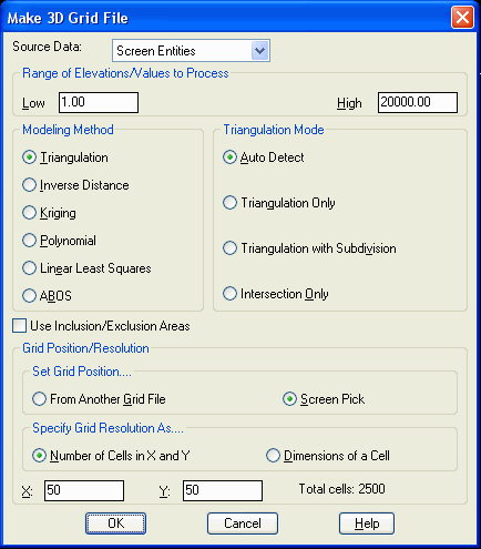
The dialog box sets the range of elevations to process, modeling method and grid resolution. Each of these items is described below.

• Source Data: This option selects the type of data to use for gridding. The Screen Entities option processes selected 3D entities from the drawing including points, lines, polylines, 3D faces and inserts. The Coordinate File and Text File options read point data from the selected file. These methods are useful for large datasets that would take extra memory and time to draw as points in the drawing. For the Text File, the program will prompt for the order of the fields and the delimiter. The Triangulation File option will interpolate the grid elevations from the selected triangulation surface.
  

• Range of Elevations/Values to Process: Entities with elevations or values outside the range to process are ignored and will not be used for the gridding.

• Modeling Method: The modeling method almost always should be triangulation for surface topographic grid files. Polynomial, inverse distance, kriging and linear least squares apply to random data points for surfaces like underground features, usually sourced by such methods as drillholes, data tables, etc.

• Triangulation Mode: When using Triangulation and Polynomial methods, There are four triangulation modes: AutoDetect, Triangulation Only, Intersection with Triangulation and Intersection Only.

• • Auto Detect method automatically chooses between the Triangulation Only and Intersection with Triangulation methods. If the selected surface entities are primarily made of polylines, then the Intersection with Triangulation method is used. Otherwise the Triangulation Only method is used.

  • Triangulation Only method builds a triangulation surface out of all the selected points, lines and polylines. All lines and polylines are treated as breaklines. Grid node elevations are calculated based on the triangulation.

  • Triangulation with Subdivision method uses the subdivisional surfaces modeling method. This option causes each triangle in the triangulation surface model to be subdivided into an average of three smaller triangles per subdivision generation. This gives a much smoother surface model, where instead of one triangle, there are now three or more.

  • Intersection Only method goes directly to the Steepest Intersection method using the selected lines and polylines. The Steepest Intersection method is used to assign the grid node elevations from the linework of the triangulation lines and the selected lines and polylines. The triangulation step is skipped and any selected point data is not used. This method can be used for making grids out of polylines such as a contour map as long as the surface is defined just by contour polylines without needing spot elevation points. Skipping the triangulation step makes this method a lot faster especially for large files.

• Use Inclusion/Exclusion Areas: This option will prompt for inclusion and/or exclusion perimeter polylines and will only assign grid cell elevations within these areas and leave the rest of the grid cells as Null.
  

• Grid Resolution: The grid resolution is specified by either the number of grid cells or by the size for each grid cell. It is usually best to set the Dimensions of a Cell to a known size, and the program will calculate the "number of cells in X and Y." While the program can handle really large grids with no limit, a general rule of thumb is to keep the total number of grids cells under 500,000 (about 700 by 700 cells) to limit the processing time. The grid location and resolution can also be specified by using the position/resolution from an existing grid file. In this case, the location and resolution of the new grid will match those of the selected grid file which is useful for routines that require two grid files with identical locations and resolutions.

No elevations are calculated on grid cells that extend beyond the extent of the data. The figure shows an example of how the grid is calculated to the limits of the data points. Extrapolation can be used to calculate elevations for the grid cells that are beyond the data limits. When there are grid cells with no elevation in a grid (.GRD) file, many routines will prompt Extrapolate grid to full grid size? Extrapolation fills in all the grid cells. The method to extrapolate uses a safe calculation that tends to average out or level the extrapolated values. So extrapolated grid areas are not as accurate as grid areas within the limits of the data. Grid File Utilities can be used to apply and save extrapolation to a grid file. The Plot 3D Grid command can then draw the grid file so that you can see the extrapolation.

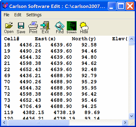
A Carlson grid (.GRD) file has the following format:

The rest of the lines are the Z values of the grid intersects starting from the lower left moving in the left to right direction and ending at the upper right. If the intersect has no value, the letter 'N' is saved instead of the Z value for Null values. An example is shown in the Display-Edit Report dialog.

Gridding from Contour Maps

A grid file can be created from contours represented as polylines with elevation. The program calculates the elevation of each grid corner by looking for contour intersections in eight directions (N, S, E, W, NE, SE, SW, NW) and then interpolating the elevation between the two steepest intersections.

To accurately model the surface, it might be necessary to add entities in addition to the contour polylines. For one, spot elevation points can be added for the high and low points. Otherwise the grid model might plateau at the last contour. Also 3D breaklines need to be added on long narrow ridge and valley contours because in these areas the program will find the same contour when it looks for intersections in the eight directions. When all eight intersections are the same contour, the interpolated grid elevation equals the contour elevation instead of rising up the ridge or dipping in the valley. The 3D breaklines force interpolation along the ridge or valley. To draw these polylines, set the OSNAP to Nearest and run the 3D Polyline command. Then draw the polyline by picking the contour polylines where the breakline crosses them. Another way to quickly create breaklines is to first draw 2D polylines. Then convert these polylines into 3D polylines with the Screen option in the 2D to 3D Polyline by Surface Model command found on the 3Dpoly menu. There is also an automatic way to draw these breaklines. Under 3D Data, use the command: Create Ridge polylines from Contours.

Prompts

Grid File to Create File Selection Dialog
Enter a name for the grid file.
Use position from another file or pick grid position [<Pick>/File]?
Pick Lower Left grid corner <8111.88,3985.08>: pick a point for the lower left limit of the grid
Pick Upper Right grid corner <8366.88,4195.08>: pick a point
Make Grid File dialog box
In this dialog, you specify the grid resolution and whether or not to include data points with zero elevations. You can specify the resolution by entering the number of grid cells in the X and Y directions. By the Dimensions option, you to set the X and Y size for each grid cell.
Reading points ...
Select points, lines, polylines and faces to grid from.
Select objects: Specify opposite corner: 1075 found
Select objects:
Reading points ... 980
Finding points on breaklines ...
Ignored 2729 duplicate points.
Inserting breaklines 3480 ...
Triangulating points ... 980
Assigning grid values> 1800
Writing grid file: C:\Carlson 2008\WORK\example1.grd
Pick the Lower Left grid corner: pick a point for the lower left limit of the grid
Pick the Upper Right grid corner: pick a point

Pulldown Menu Location: Surface
Keyboard Command: mkgrid
Prerequisite: Entities that define the surface