This lesson will step through some of the more common Hydrology module routines, and design structures based on the analysis of the watershed. To load the Hydrology module, run Settings->Carlson Menus->Hydrology Menu. The drawing file HydroLesson.dwg is a nice example to show the features of the Hydrology Module. A surface hydrolesson.tin file is needed for these routines, and is supplied also.
Open HydroLesson.dwg. After opening the drawing, take a look around at the various layers, and then go to the 3D View Window under View, to see the change of elevations in the surface.
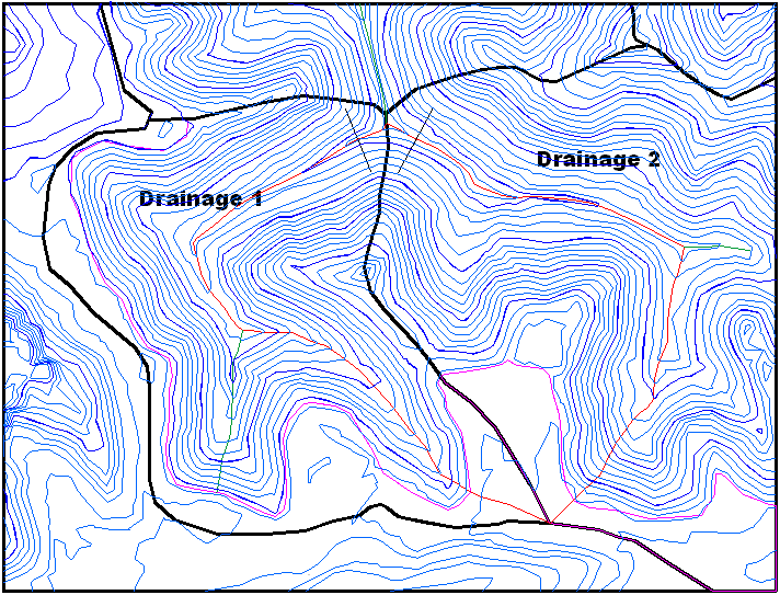
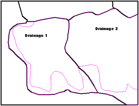
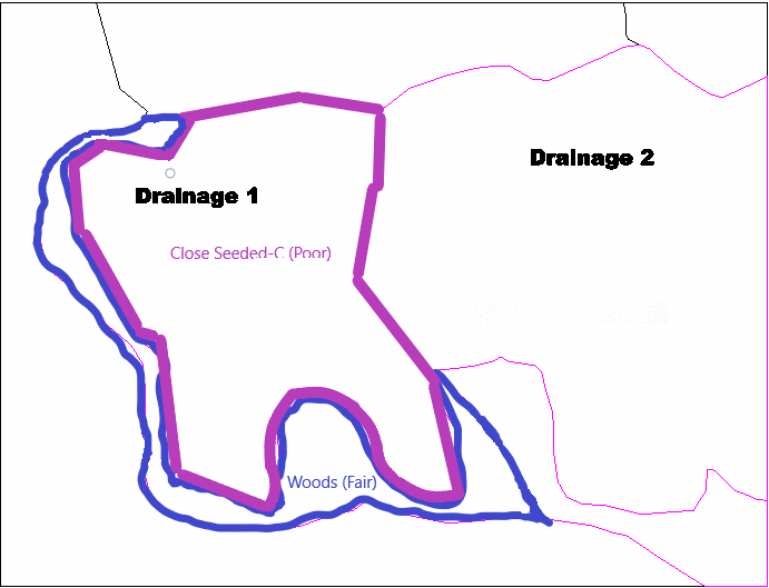
There are two main drainage areas that we will be looking at: Drainage 1 and Drainage 2. They are labeled in the below graphic. The other drainage areas in this region will be ignored, as they do not drain to the same area we are looking at, the north central low spot.
There are routines for finding these watersheds based on grid or
TIN files, but this drawing has the closed polylines already
generated.
We will walk through some of the steps to gather the slope and area
information.
Step 1
Slope Report.
Go to View and use Freeze Layer to freeze all contours, which
are on two separate layers.
We will run the following routine twice, once for each
watershed.
Go to the Surface pulldown menu in the Hydrology module.
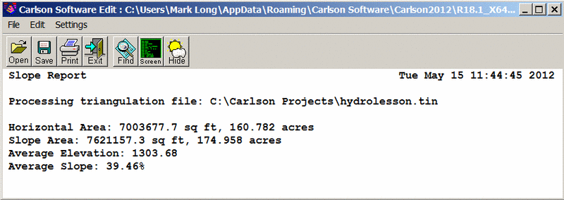
From the Surface menu, choose Slope Report.
Choose the Slope report by area option, which is the default, and
you will be prompted for File or Screen.
Choose File, and notice that we have the Hydrolesson.tin file,
found in the Carlson Projects folder, to analyze. Open it.
When prompted for the inclusion line, select the closed perimeter
line that runs around Drainage 1.
Press Enter for none when prompted for the exclusion line.
The report window will appear, and the information can be saved to
a file, placed on-screen, or simply reviewed here using the Carlson
Standard Report Viewer.
In this example, we will review the reports in the viewer.
Next, analyze and report on the Drainage 2 watershed, again using
Hydrolesson.tin.
Shown in the following figures are the reports of the two drainage
areas.

Step 2
Run Off Tracking.
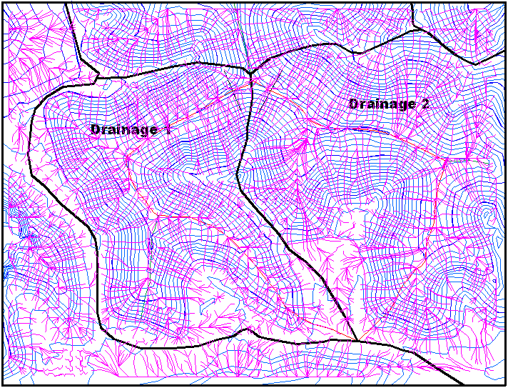
The command Run Off
Tracking is found under the Watershed pulldown under
hydrology . It will draw a 3D polyline running downhill in the path
that a storm event would. It is useful to fine-tune a watershed
boundary. If you pick near the boundary line, you can see which
direction the water will flow.
Shown is an example of the drawing with the runoff tracking lines
falling within their respective watersheds.
Step 3
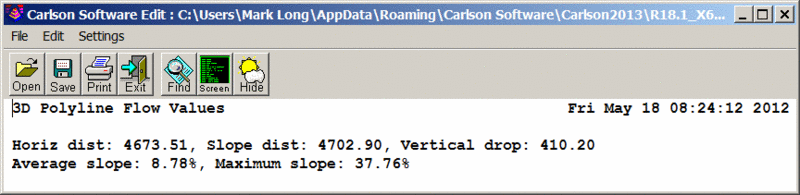
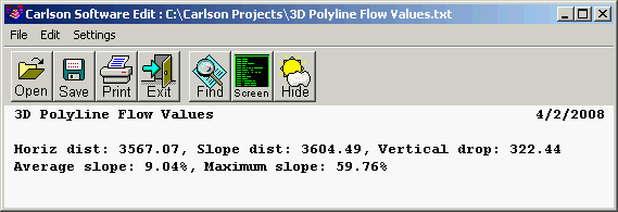
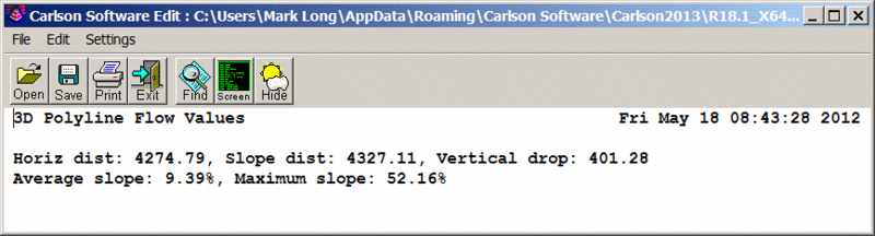
3D Polyline Flow Values.
This is a step to see what the longest flow line data is within the
watersheds. It will create a nice report showing the slopes and
vertical drop.
The 3D polylines in the drawing were created (with runoff tracking
and some editing) to represent the longest flow line.
This routine reports out the values of the polylines
selected.
Go to the Watershed pulldown to Report flow values or flowvals on the command
line.
The report can be saved for future reference,
but also be aware that when you will need to enter in this
data,
there is a button on the dialog to simply pick the polylines
on-screen.
Step 4
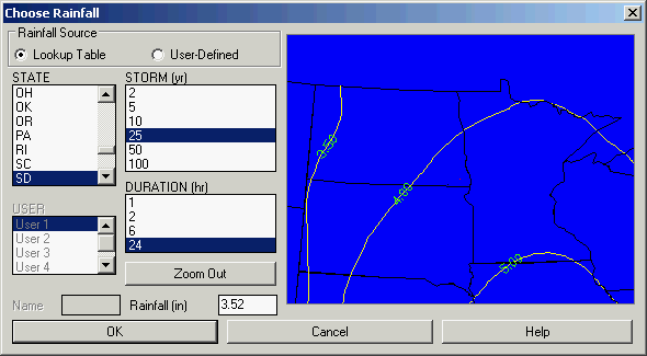
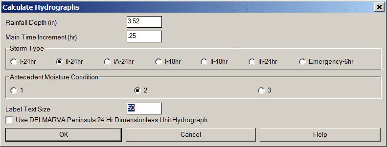
Rainfall Frequency & Amount.
This routine will look up rainfall depths based on
what storm type and duration is being analyzed.
Under Watershed, go to Rainfall
Frequency & Amount TP -40 TP -47. We will do the 25
year, 24 hour storm.
Let's assume the area is somewhere in South Dakota, and so we will
use the value of 3.52 inches.
For customizing this table to suit your needs, there is the
user-defined portion in the lower left corner, if you have specific
values you always use; they can be entered here for quick
retrieval.
Step 5
Sub-Watersheds by Land Use.
This is another way to break up the watersheds, based on land use,
or varied surface features.
We will break up our watersheds into two types of land use.
The steep slopes will be treed, and the top flats will be vegetated
with grasses.
Go to Sub-Watersheds by Land
Use under the Watershed pulldown.
The routine will then ask for the watershed boundary, pick the two
closed polylines that make up the two different areas. Pick the
lines as prompted. The two lines are drawn in layer PILLARS so that
the program knows how to identify them.
Step 6
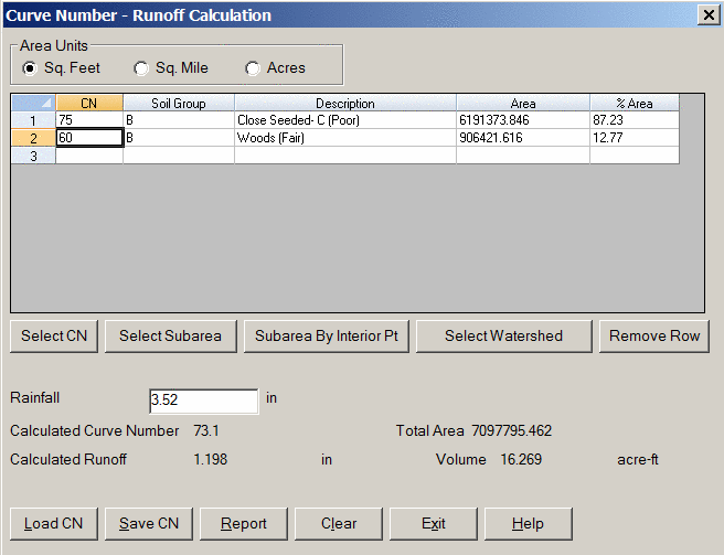
Curve Numbers (CN) & Runoff.
This is an easy step to get the runoff and volume of the storm
based on the CN and acreage.
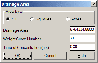
We will do a weighted curve number representing two land use
types.
We will run this twice, once for each watershed. Go to Curve Numbers (CN) & Runoff under
the Watershed pulldown.
First off, Select Areas, and pick the two closed polylines lines
just created inside Drainage 1 (the PILLARS layer).
They will have two different CN, based on the type of land.
The area is brought in automatically, and the CN will have to be
typed in, or looked up on the table.
For this example, type the information in according to the charts
below.
After the CN numbers and the areas are in, hit the Calc Runoff
button, and the runoff and volume will appear at the bottom.
These can be saved in a report, or simply written down for future
reference.
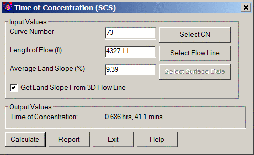
Drainage2

Drainage 2
Step 7
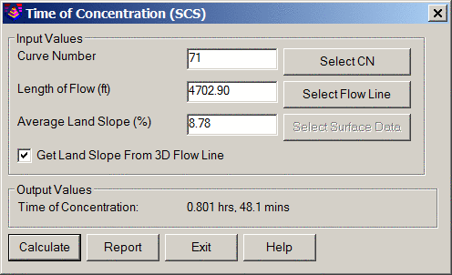
Time of Concentration (Tc).
This is a quick step necessary for ultimately
getting the Peak Flow.
Under Watershed, go to Time of Concentration
(Tc).
We will use the SCS method, and the window will look as
follows.
The CN number should have been brought in from the last routine,
but we will have to Select Flow Line from Screen.
This will allow for picking the flow line from the map.
This routine will also be executed twice to calculate the TC for
both drainage areas.
Drainage 1
Step 8
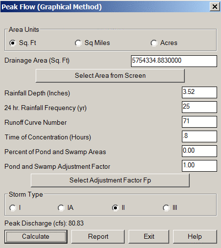
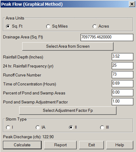
Peak Flow (Graphical Method).
Now, let's see what the peak flow will be in each
drainage, based on the previous seven steps.
Run Peak Flow->Graphical Method from the Watershed pull-down
menu.
The drainage area of the last watershed calculated should appear in
the Area window.
If not, then simply type it in. The Rainfall depth, frequency, CN,
and TC also should be there.
All we have to do is hit Calculate, and the peak discharge appears
at the bottom in CFS (cubic feet per second).
This routine should be run twice, once for each drainage.
Notice that all of these routines have a Report button to keep a
running log of all the calculated data.
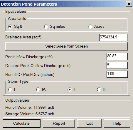
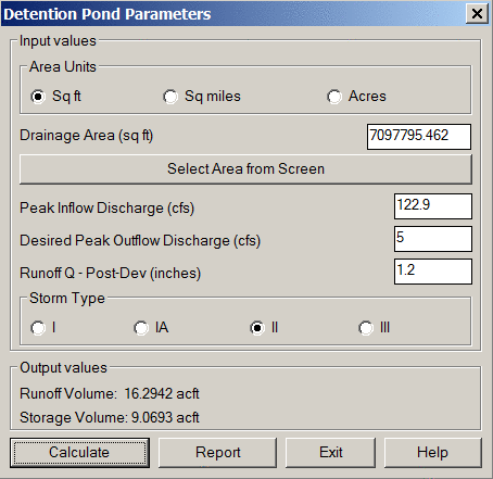
Step 9
Detention Pond Sizing.
Now we need to see how large the ponds need to be
to detain this size of a storm event.
Under Structure, go to Detention
Pond Sizing > TR-55
Method.
The Peak Inflow Discharge from the last area calculated will
appear, as well as the area.
In this example, we will allow for a combined maximum 10 CFS
to be discharged from the ponds.
This means that 5 cfs from each will be our Desired Peak Outflow.
Type that in.
Hit Calculate, and the Runoff Volume and the Storage Volume will
appear at the bottom of the window.
In pond number one, we need to store 6.68 acre feet of water.
In pond number two, we will need 9.07 acre feet of storage. So now
we have a starting point, and we can now create the pond in 3D with
these sizes.
Step 10 Design
Valley Pond.
We know approximately where we want the two ponds, and have the dam
polylines drawn in the drawing already.
They are in the top-of-dam layer. If it is frozen then thaw it out
now.
run Design Valley
Pond found under the Structure pulldown
menu.
For pond number one (corresponding to Drainage 1), the values to
enter at each prompt are:
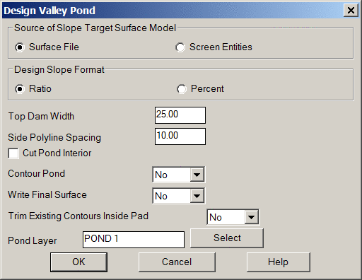
Pick the top of dam polyline:
pick it
Select Existing Surface dialog:
Open the hydrolesson.tin file
Pick a point within the pond:
pick a point upstream from the top of
dam polyline
Enter the outslope ratio <2.0>:
2
Enter the interior slope ratio
<2.0>: 2
Range of existing elevations along dam top:
1075.88 to 1172.06
Enter the top of dam elevation: 1109
Calculate stage-storage values
[<Yes>/No]? Y
Method to specify storage elevations
[<Automatic>/Interval/Manual]? I
Starting elevation <1088.96>:
1088
Elevation interval <2.00>:
press Enter
A Valley Pond Report is produced. Review it noting the stage at
which our target storage volume is eclipsed and exit out.
Output grid file of final pond surface
[Yes/<No>]? press
Enter
Write stage-storage to file
[Yes/<No>]? Y
This will be a *.CAP file, name it pond1.
Adjust parameters and redesign pond
[Yes/<No>]? N
Trim existing contours inside pond perimeter
[Yes/<No>]? N
Contour the pond [<Yes>/No]?
N
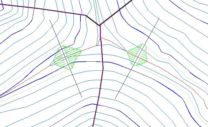
You should now have a pond that looks like the one on the left in the following drawing. Repeat the routine for Pond 2, using a top of dam elevation of 1087, and starting at a low of 1065.
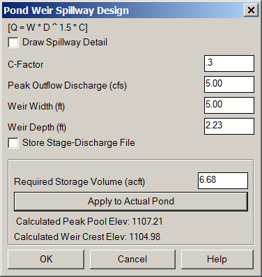
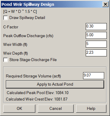
The C-factor we will use is about .3. We will allow up to 5 CFS discharge. This will calculate the depth of the weir (if that is what we use, we'll use a drop pipe in 1, and a channel in 2) with the equation shown at the top of the window. Our required storage volume is 6.68 acre-feet for pond one (9.07 acre-feet for pond two). Hit the Apply to Actual Pond and choose the Pond1.cap stage-storage capacity file output from step 11. This should give the two elevations shown in the dialog: 1106.73 for top of pool, and 1104.50 for bottom of spillway. This will be our principle spillway. Our emergency spillway will just be assumed to be 1.5 feet higher.
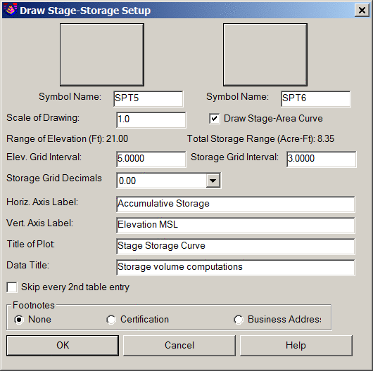
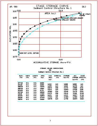
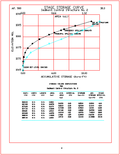
Step 12 Draw Stage-Storage Curve. Now that we have the spillway elevations and a capacity file (*.CAP) for each pond, let's draw the Stage Storage/Area Curve Graphs to get a graphic of the curves with values to follow. Under Structure, go to Stage-Storage, and then slide over to Draw Stage-Storage Curve. Below the following dialog box are the settings to be entered for Pond 1:
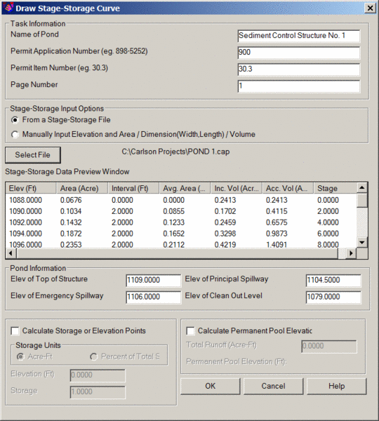
Click OK.
Pick Starting Position: pick a spot in the open drawing
Do the same for Pond 2, with the other elevations from the
spillway and top of dam calculated above, and choose to put this on
Page Number 2. Your graphs should look like the two
pictured.
Drainage 1
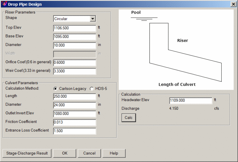
Step 13 Drop Pipe
Spillway Design.
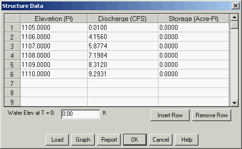
This will give us a stage discharge file that we will add to our structure in the routine of the storm through our ponds. We will only do this in pond 1. Pond 2 will have a channel, which will create a different stage discharge file. Go to the Structure pulldown to Drop Pipe Spillway Design.
We will design one for the flow we need. Enter in the values shown in the window and hit calculate to get near the 5 CFS discharge we are looking for. Hit File to create the discharge file for pond 1.
Step 14 Channel Design (Manning's n) Non-Erodible. This will generate the other stage discharge file for pond 2. Go to the Structure pulldown to Channel - Non-Erodible. Enter in the parameters shown, and create the second STG file, this one for pond 2. It will calculate the depth and the velocity, based on our dimensions entered.
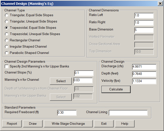
Click Write Stage-Discharge. You will then provide a file name for the new STG file and save it. It will calculate the depth and the velocity, based on our dimensions entered. Enter a depth of 1.5 and a base elevation of 1081.95 for the bottom.
Step 15 Draw Flow Polylines. Now we will look at creating a skeleton structure of our flow lines with these structures placed on them. We will first produce a hydrograph of the two drainages without the ponds, then add the ponds to the flow polylines and regenerate the hydrographs. We hope to reduce the discharge to a much smaller amount, but over a longer period of time.
Under Watershed > TR-20 Routing, go to Draw Flow Polylines. This will let us pick a point, from high to low. As seen in the diagram, pick from NW to SE. Enter in the three parameters for Drainage 1.
When asked to draw another, select yes, and join it with the first at the bottom right corner, near the endpoint. This will place the text on them and allow for the next step.
Step 16 Hydrograph Development. This routine will run the TR-20 program and generate a hydrograph file that we can draw on screen. Under Watershed > TR-20 Routing, go to Hydrograph Development and select the two Flow Polylines and the text associated with each one.
The routine will run the TR-20 and give a Standard Report Viewer report. There are now some hydrograph files created in the data directory that we can draw in the next step.
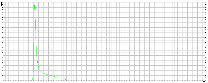
Step 17 Draw Hydrograph. Under the Watershed pulldown, go to Draw Hydrograph and select the J1ADD.h1. This is the file of both drainages combined.
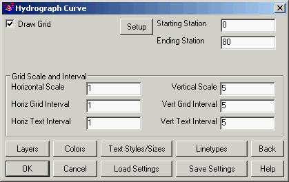
The scales to be used should be about 1,1,1,5,5,5 and we will draw the grid on the first one, and turn off grid for additional hydrographs. Choose starting time of 0, and an ending time of 80 (the next one will go that long).
Step 18 Locate Structures. The Locate Structures command, located in the Watershed > TR-20 Routing menu, will place a symbol on our flow lines to representing the ponds and spillways. This will create a small triangle at the end of each flow line where they were picked. You will run this on each flow line individually.
Hit the Load button twice: once to pick the (pond1 and pond2) CAP file and again to pick the STG file. Finally, after you hit OK, you are now ready to run Hydrograph Development again to generate the new hydrographs.
This completes the tutorial: Hydrology and Watershed Analysis.