Basic Road Design with Volumes
This tutorial requires
the Civil Design program.
1
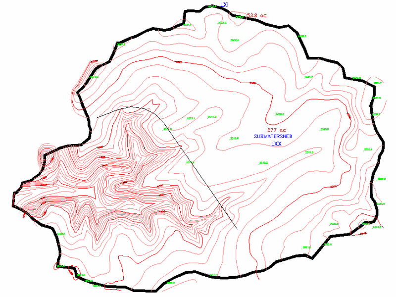
First we need to open an example drawing
supplied with Carlson.
under the File menu click on Open command and choose
EXAMPLE2.DWG.
It should be in the Carlson Projects folder, and will look like the
example (without the curved road).
2 Draw Road
Centerline.
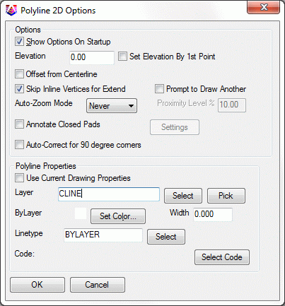
Issue the Draw > 2D
Polyline command and generate the road centerline shown
below. If the Polyline 2D Options dialog box appears,
provide the values as shown below and then click OK.
[Continue/Extend/Follow/Options/<Pick
point or point numbers>]: 1857700,159400
[Arc/Close/Distance/Follow/Undo/<Pick
point or point numbers>]: D
Enter Distance
[Meters/<Feet>/Chains/Links/Rods/Pick/Quit]: If Feet is
not in < > click on feet
Enter distance: 310
Define direction method
[Cursor/Line/<Angle>]: press
Enter
Code: 1-NE 2-SE 3-SW 4-NW 5-AZ 6-AL 7-AR
8-DL 9-DR
Enter angle code (1-9) <7>: 1 (for a northeast bearing)
Enter bearing (dd.mmss):
68.5525
Enter Distance
[Meters/<Feet>/Chains/Links/Rods/Pick/Quit]:
Q
[Arc/Close/Distance/Extend/Follow/Line/Undo/<Pick
point or point numbers>]: A
[Radius pt/radius Length/Arc
length/Chord/Second pt/Undo/<Endpoint or point
number>]: L
Specify radius length:
500
Curve direction
[Left/<Right>]: press
Enter
[Arc length/Chord length/Delta
angle/<End point or point number>]: D
Specify delta angle (ddd.mmss):
76.2405
[Arc/Close/Distance/Extend/Follow/Line/Undo/<Pick point
or point numbers>]: L
<Enter or pick distance>:
1663.2721
[Arc/Close/Distance/Extend/Follow/Line/Undo/<Pick point
or point numbers>]: press
Enter
3
Polyline to Centerline File.
This step will create a centerline file necessary for the final
road design routine. We will do the simplest variation, which is
simply picking a polyline. There are other methods to design a
centerline. They are documented in the manual.
First (if necessary), zoom back to the extents of the plan view,
as we will be working with the polyline created above. Go to
Polyline to Centerline
File command, under Centerline, and name a *.cl file to
create.
Polyline should have been drawn in
direction of increasing stations.
Select polyline that represents centerline: pick polyline
representing the centerline
Centerline station [Reverse/Ending/<Beginning: 0+00>]:
enter
Station    North(y)     East(x)      Description

---------------------------------------------------------

0.000      159400.000   1857700.000  LI

310.000    159511.480   1857989.262  PC

976.728    159329.389   1858580.264  PT

2640.000   157961.527   1859526.534  LI
Press ENTER to continue.
press Enter
4
Profile from Surface Entities.
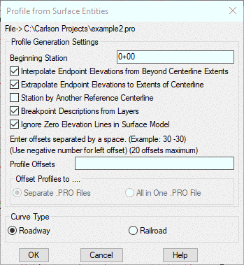
Now we will make a profile file, *.pro. This will be
from the centerline shown in the drawing as the line with the
curve.
Under the Profiles menu choose Create Profile From... then
Profile from Surface
Entities.
This will create a new file. Type in a file name in the dialog and
click Save.
On the next dialog, we will use the default values and click
OK.
Pick the centerline, and without hitting enter, type all. The
data is written to file.
NOTE: Common practice is to build a surface
model from any and all data that carries an elevation. However,
there are several Carlson Create Profile from... routines
and we'd like to work with a routine that gets its information
"direct from the source" (i.e. the contours
themselves).
5
Draw Profile.
This will give us a profile view of the contours at our
centerline.
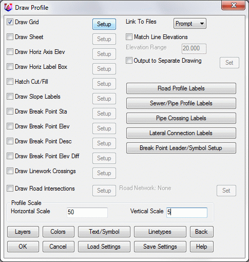
Under Profiles, go down to Draw
Profile and add our new file to open. Click Ok
.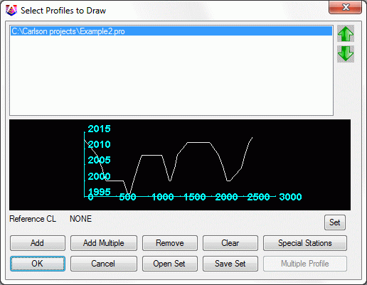
The window below will appear as shown. With the horizontal scale
set to 50 and the vertical scale set to 5, there will be a 10X
vertical exaggeration of the profile. Fill this dialog box it out
as shown below and click OK
.
Next, there is the Profile Grid Elevation Range dialog.
Accept the top and bottom elevations it gives by hitting OK.
Pick a spot in the drawing to draw the profile,
then view the profile on the grid by zooming as required.
Your profile should look similar to this.
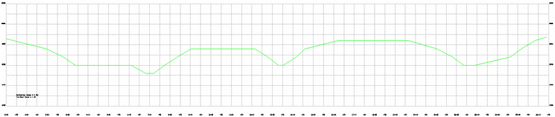
NOTE: The "flat spots" shown in this profile
are the result of extracting the profile data directly from the
contours. Extracting a profile from a surface model is a more
common approach in today's computer age.
6
Design Road Profile.
Now we will design how the road centerline profile will be,
in relation to the existing ground (which is the first profile we
have made).
This routine will create another Profile file.
Under Profiles Menu,
go to Design Road
Profile< Design Road On
Profile Grid (this method is suggested for this
tutorial).
The following dialog box will appear. Since we followed up the
Draw Profile command with
this one, it was able to determine proper startup values for the
dialog.
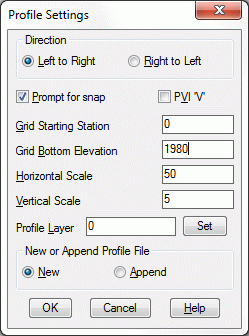
Choose OK on this dialog. A new file creation dialog box will
appear, asking for an output file name. Enter a name such as
DESIGN, and click Save.
Pick Lower Left Grid Corner
<0.00,0.00>[endp on]: pick
the lower left grid corner of the profile grid
Carlson has endpoint osnap active to make the pick accurate
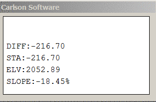
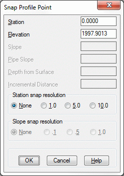
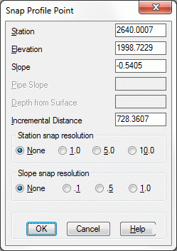
At this point another dialog will appear in the upper left
corner.
Initially, it will display only station and elevation.
Once a beginning point has been designated, it will also display
the relative difference from the last point to the cursor position
(illustrated below).
This can be an aid in determining acceptable slopes for your
design.
Enter a station or pick a point (Enter to
End): END
of pick the
left-most endpoint of the existing ground profile as a tie in
point
The following dialog appears. Choose OK to accept the
defaults.
Station of second PVI or pick a point
(U,E,D,Help): 1111.01
Percent grade entry/<Elevation of
PVI>: 1999.37
Station of next PVI or pick a point
(U,E,D,Help): 1911.64
Percent grade entry/<Elevation of
PVI>: 2002.66
View table/Unequal/Through pt/Sight
dist/K-value/<Vert Curve Length>: 500.00
For Sag with Sight Distance>VC and Vertical
Curve => 500.00
Sight Distance => 1000.0, K-value =>
306.6 [1793.8]
Use these values (<Y>/N)? Y
Station of next PVI or pick a point
(U,E,D,Help): END
of pick the
far-right endpoint of the existing ground profile as a tie in
point
The following dialog appears. Choose OK to accept the
defaults.
View table/Unequal/Through pt/Sight
dist/K-value/<Vert Curve Length>: 500.00
For Sag with Sight Distance>VC and Vertical
Curve => 500.00
Sight Distance => 1000.00, K-value => 697.0
Use these values (<Y>/N)? Y
Station of next PVI or pick a point
(U,E,D,Help): press Enter
At this point the following dialog appears. Change settings to
match, and choose OK.
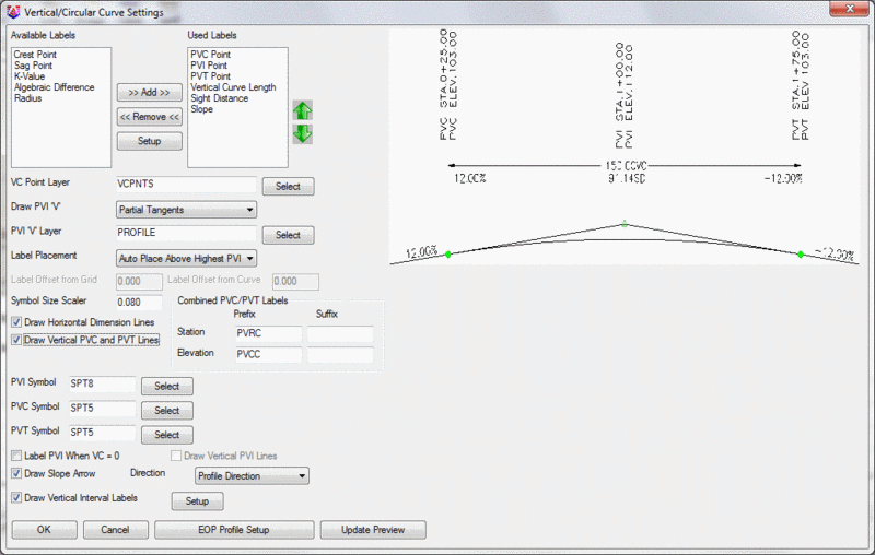
Pick vertical position for VC text:
if prompted pick a point above the top of the
grid
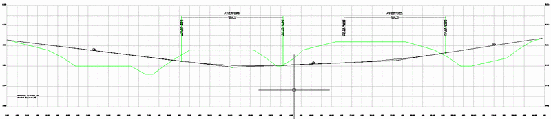
Carlson will now finish the road design, and your drawing should
like the following:
7
Input-Edit Section Alignment.
Now we will layout the alignment for our cross-section file. This
step gives the section interval, and the offset left and right from
our centerline.
Under Sections, go to Input-Edit
Section Alignment. Choose the New tab, which brings up the
dialog to make a new MXS file (multi-xsection file). Type in a new
name and click Open. Notice how all files can have the same name in
this road design portion, as they all have a unique file extension.
So for the organization of various jobs, it is sometimes helpful to
have all of the files with the same name.
Polyline should have been drawn in
direction of increasing stations.
CL File/<Select polyline that represents centerline>:
pick the centerline polyline
Enter Beginning Station of Alignment
<0.00>: press Enter
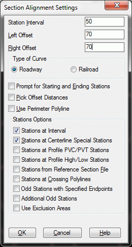
The dialog will appear as shown, enter in the stations and
offsets exactly as they appear here. This will give the needed
detail for the road design routine.
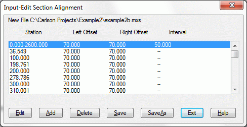
Choose OK, and another window appears that allows for any
station editing or changes. It all looks good here, so hit
Save.
The Alignment file is now written. There is now a preview of the
section alignment lines shown on the centerline. These are just
images, if the drawing is regenerated, they will disappear (they
can be drawn permanently if desired).
8 Sections
from Surface Entities. Next, we will create the actual section file
(*.SCT) from the contours, in combination with the alignment file
(*.MXS).
Under Sections > Create Sections from..., go to Sections from Surface Entities. We
will use the contours and breaklines for surface elevations, as we
did with generating the profile.
Specify the MXS file that we just created to read for the
alignment. Click Open to select it. Then choose a new file name for
the section file, and click Open.
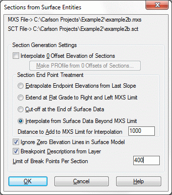
We'll enter in a distance of 1000 feet to add to our MXS limit
of 70. This will search farther for contour elevations, then choose
OK. Now, select the surface entities which are the contours and the
breaklines. Once you are back to the command prompt, you are done
with the making of sections.
9
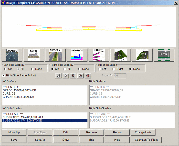
Design Template.
Let's design a wide boulevard, 30' of drivable pavement, with curb
and gutter on the outside. Whenever a cut is within rock, the cut
slope will employ a 0.5:1 slope rather than the typical 2:1 slope.
At the top of rock, the cut will revert to 2:1. In fill, the
condition will be 3:1 for fill under 6' and 2:1 for fill over 6' in
depth. Pavement depths will be 8" of stone and 4" of asphalt.
First, Select Design
Template, found under Roads, within the Civil Design module
of Carlson. Click on the New tab.
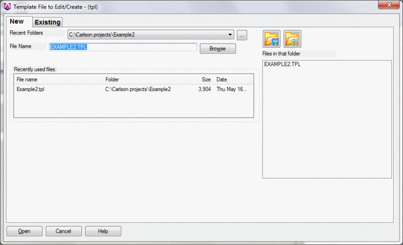
We'll give it the same name as the drawing. Choose Open. A large
dialog box appears as shown below. In it, you enter segments of the
template, which work outwards from the middle as you add more
lanes, curbs and shoulders. We will enter a symmetrical
template,
with 13.5' pavement sections either side of centerline,
connecting to a 2' curb and gutter,
with 18" of gutter and 6" of curb.
Then we'll add a 6' shoulder.
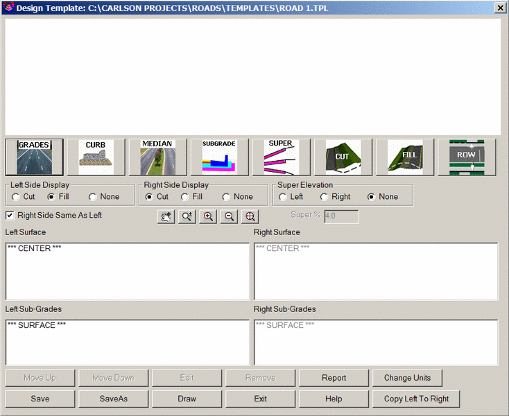
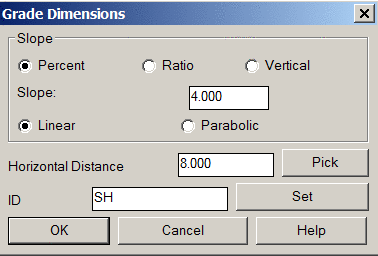
For the lanes, click the Grades icon. This leads to a child
dialog as shown next:
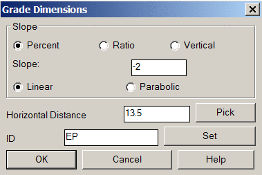
Fill out as shown. It's important to note that a downhill pavement
from a crown in the middle is entered as a negative slope.
That is, it is 2% heading from centerline outward, regardless of
which side of centerline we are speaking of. Slope is in reference
to the centerline of the template,
and it is independent of the profile grade point. It is also
important to enter an ID whenever requested. ID's can be referenced
later.
A break point in a shoulder in superelevation could be defined
as occurring at EP+3, as opposed to the exact offset distance from
centerline. The advantage of EP+3 is that if the road lane width
expands (e.g. for a passing lane), but the shoulder always breaks 3
feet beyond edge of pavement, then EP+3 is the only effective way
to reference the break point. Now click OK. You'll note that the
lanes show up in the preview window at the top.
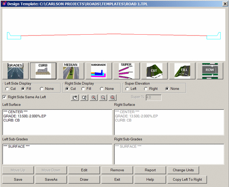
Next, we will add a curb. Click the Curb icon. Fill out as
shown:
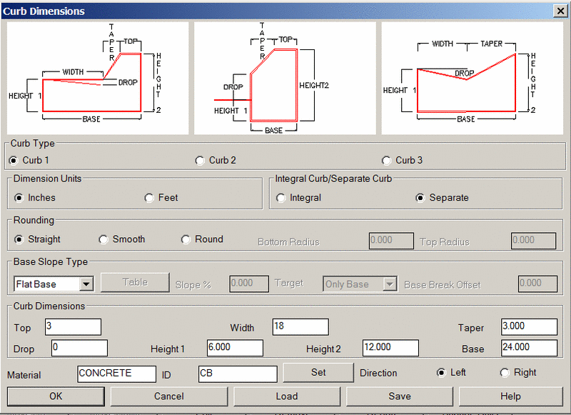
It is especially a good idea to match crown -- to make the curb
match the slope of the last pavement lane (2% above). But if your
curb tilts downward more (like 3%), then use a Special Base Slope
Type. If it is flat, by all means click on Flat Base. Now click OK.
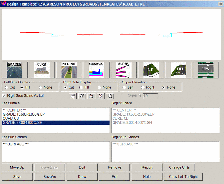
Here's what our screen looks like so far:
Next, we will add a shoulder, going uphill at 4% for 8'. Notice
what is happening. You are lit up on the Curb line, so if you add
another Grade, it will append after the curb, and add to the back
of the curb. If you were to click on the GRADE: 13.500, -2.000%, EP
line, then click on GRADES, you would add a second lane before the
curb, which is NOT what you want. Now click on GRADES with CURB: CB
highlighted. Fill out the dialog as shown:
That's it for the surface! Here's what our screen looks like
now:
Note as you select the different items as you create them, the
viewer window will highlight the selection.
Now we have subgrade and outslopes still to consider. Let's turn
our attention to subgrade. Let's think about this: if our pavement
is a total of 12" deep (4" asphalt, 8" stone) and our concrete
gutter is 6" deep, then the stone will run 6" deep under the
gutter. Do we want this stone to come back up at the back of the
gutter, behind the gutter, or even wrap around back into the
gutter, like a layer of bedding that is covered by dirt? The most
complex concept is the wrap around, so let's go for it.
Select the Subgrade icon. We'll do two subgrade surfaces: first
asphalt, which will run straight out and hit the curb, and then
stone, which will run out, go under the curb, and wrap back.
For any sub-grade, we still do the vertical offset as a negative
distance (negative meaning down). But follow this concept: we start
it out 13 feet from offset 0, and keep going at "Continue Slope"
until it hits something (the curb). This won't work if there is
nothing to hit. But it will run into the curb. Or if there is a
fill slope, downhill 6:1 recovery zone lane, or something to
intersect, it will also. This Continue Slope concept works
perfectly for shallow asphalts and concretes that will bump into a
curb, when extended.
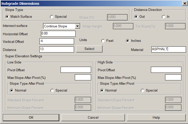
Complete as shown above, and click OK.
Now for the other subgrade: the stone beneath the asphalt.
Follow this: if the stone can't Match Surface (note this option
under Slope Type), it will start uphill with the shoulder as it
passes beyond the curb (it goes out 17'). So it must have a Special
Slope Type, the same 2% all the way. The Wrap Height is the
vertical rise at the end of the 17', before it wraps back and hits
the curb. Select the Subgrade icon again.
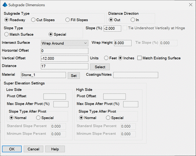
Fill out the Sub-Grade Dimensions dialog as shown above and then
click OK. Note the preview screen:
We still need to enter the outslope conditions. They are done
with the Cut and Fill icons. Fill is easy in our example. Click on
Fill.
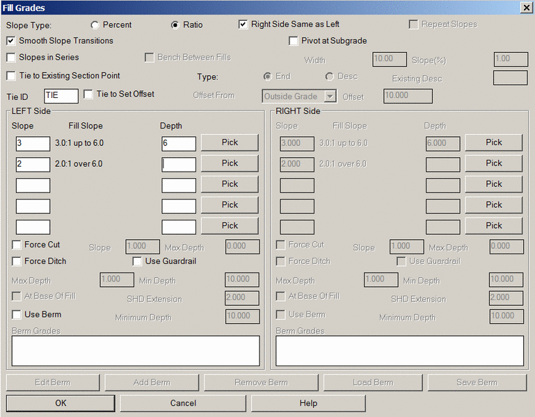
Just 3 entries total: 3 (for 3:1), 6 (up to 6'), then 2 (for 2:1
over 6'). Click OK. Next, click the icon for Cut.
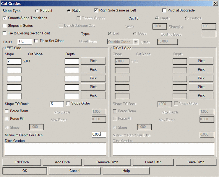
This is actually easier (in terms of total entries). Just 2
entries do it: 2 (for 2:1 normal cut) and down below, 0.5 (for
0.5:1 cut when in rock). Click OK.
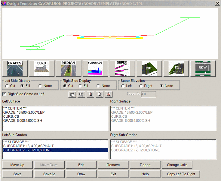
The template is complete, so click Save, and then Exit the
dialogue. Now let's prove we have a good template by doing the
command Draw Typical Template. under Roads
10 Draw Typical Template.
The file extension for templates will be tpl. Select Draw Typical Template under the Roads
pulldown menu,
select Example2.tpl (or as named above), choose Open and the
following dialog shown here is displayed:
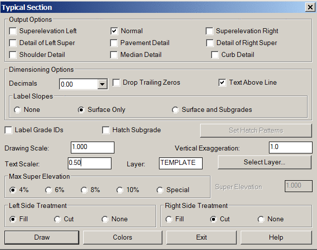
We have doubled the text scaler to 0.5 for better appearance in
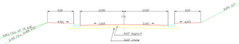
this tutorial. Click on Draw, and pick a starting position point.
Here is the look of the plotted template.
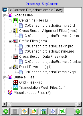
11 Drawing Explorer. As
more files are created, edited, loaded and reviewed within a work
session, the drawing ini file takes note. You can review your
active files as you work, or days later, because they save to the
ini file that shares the same name as the drawing file. To see the
files associated with this tutorial drawing file, select
Drawing Explorer by
sliding over from Project, under the File menu.
12
Input-Edit Section File.
Input-Edit Section File has many uses.
One of them is to translate or lower the elevations of a file and
re-save.
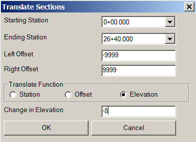
If we lower the elevations of our ground sections 8 feet, we can
call that the rock line.
Rock lines react with templates and profiles to create rock cuts
and rock quantities,
within the final step, which is called Process Road Design (Step
13).
Select Input-Edit Section
File under the Sections pulldown menu.
Under the Existing tab section, select the SCT file you created
earlier and click Open.
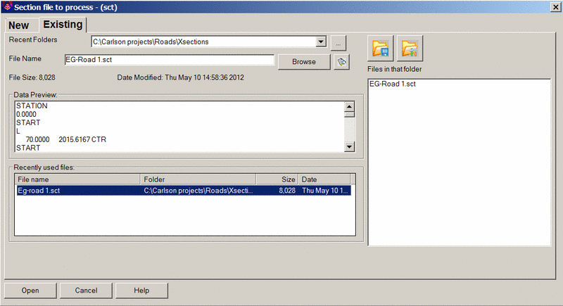
The next dialog that appears is shown below:
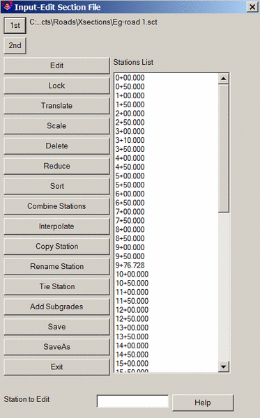
Click the Translate button. The Translate Selections dialog
appears.
The Ending Station might differ from what is showing here, but it
should be close to this value.
Make sure the rest of the dialog looks that same as shown below,
and click OK.
Now back at the Input-Edit Section File dialog, click
SaveAs,
and enter a different name, such as Example2-rock, and save the
file.
Then click Exit.
Input-Edit Section can do much more through the Edit
option.
in the case of Edit, you would first highlight one station, then
click Edit to review and revise it.
13
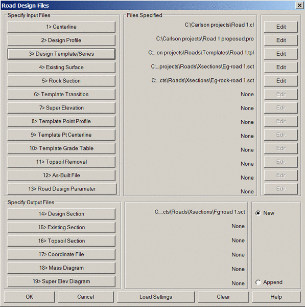
Process Road Design.
This is the routine that weaves everything together.
Select Process Road
Design, as the lower command under the Roads pull-down in the Civil Design
module.
Fill out the dialog as shown below. Be sure to select, under
Specify Output Files,
the Design Section File option and click New. Enter a new file name
and Save. Then click OK.
On the next dialog, be sure to click on Triangulate &
Contour at the lower left of the dialog.
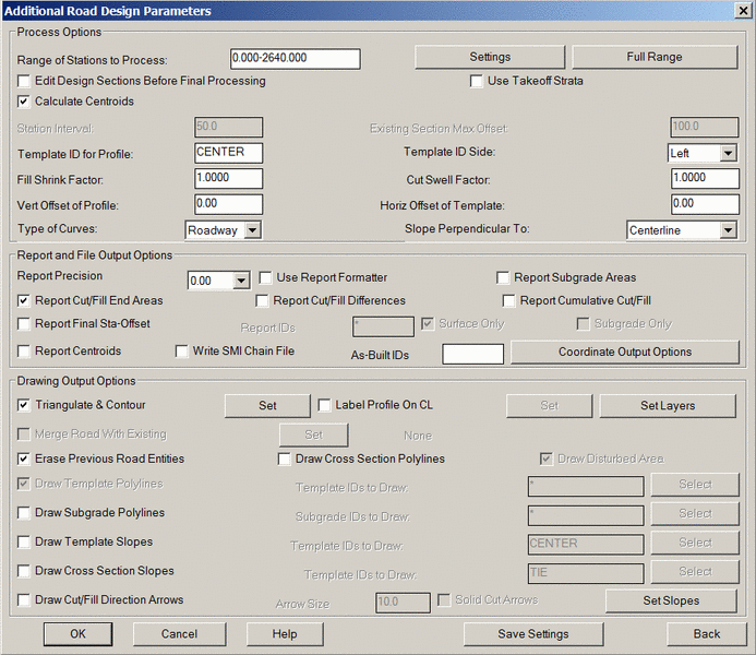
Now click OK. Here is a partial view of the final report, with
itemized quantities:
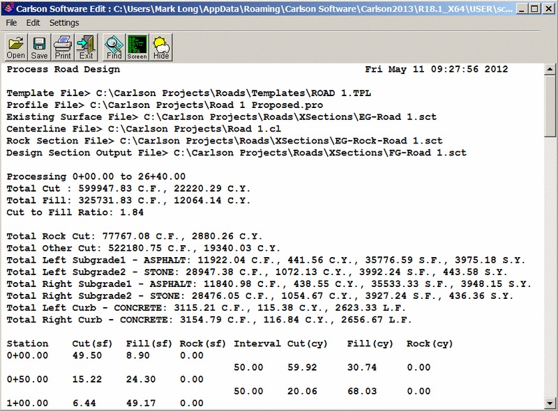
Click Exit when finished reviewing the report. You will get this
command prompt:
Trim existing contours inside disturbed
area [Yes/<No>]? Y
Retain trimmed polyline segments
[Yes/<No>]? press
Enter
Here is the resulting graphic, in 3D, obtainable by using
3D View Window found under
the View pulldown:
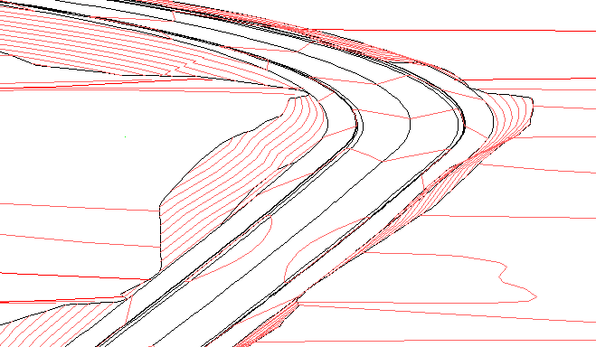
This completes the Lesson 10 tutorial: Basic Road Design with
Volumes.