There are a variety of Tools for working within
the SurvNET project manager.
From left to right/top to bottom, the tools are:
EDM Calibration - offers an option to enter field measurements
and calibrate to a published base line.
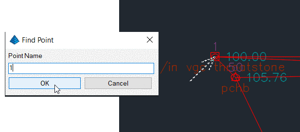
Point Search - Searches for points by
name
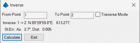
Inverse - calculates the direction and horizontal distance
between two points
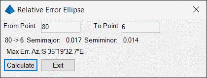
Relative Error Ellipses - calculates the error ellipse between
two points
Conversion Tools - converts data
formats of raw input files
The EDM Calibration program allows a surveyor to enter and process the raw data collected on an EDM calibration baseline. The purpose of an EDM calibration is to determine if the EDM is measuring within standards. The program performs a statistical analysis of that data as outlined in "Use of Calibration Base Lines", by Charles J. Fronczek, NOAA Technical Memorandum NOS NGS-10. The NGS document can be downloaded from the NGS website. NGS maintains a webpage on EDM Calibration Base Lines. The manual and other information on EDM calibrations can be found at https://www.ngs.noaa.gov/CBLINES/calibration.shtml. Following is the main EDM Calibration dialog box. NGS publishes the EDM calibration data in metric units. SurvNET's EDM calibration program currently expects the data to be collected in meters.

The basic flow of this program is to first fill out the lower portion of the dialog box which contains different text fields, EDM constant values, and the optional Atmospheric Corrections settings. Next, fill out the grid in the upper portion of the dialog box. This grid contains the field data collected and also the published distances between monuments of the baseline. After this information has been filled out use the 'Compute' button The program will then display the result of the calibration in the window in the lower portion of the dialog box as follows.

After the file is processed, the results can be stored as an ASCII text file. Use the Save Output or the menu option "File/Save Results File As..." to save the results. First, you will be prompted for an output file name. The input data can also be stored. Once stored it can be opened and processed again.
Following is the entire output with a brief explanation of the results. Comments about the results are inserted in bold:
EDM Calibration Report

        Observed Data

EDM Type:
Date:   Time:
Prism description:
Weather description:
Comment:
Atmosphere Correction: OFF
Constants: Refrector: 0.000   EDM: 0.000
From         From     From    To    .      To       To                      Observed    Published
Sta.         Elev.    HI      Sta.         Elev.    HI     Temp. Pressure   Slope Dist. Dist.
 STA_0        47.494  1.576    STA_150      44.631  1.552    0.0    0.0      150.0326   150.0008
 STA_0        47.494  1.576    STA_400      41.497  1.537    0.0    0.0      400.0229   399.9772
 STA_0        47.494  1.576    STA_1100     41.431  1.519    0.0    0.0     1100.0203  1100.0001
 STA_150      44.631  1.570    STA_1100     41.431  1.519    0.0    0.0      950.0081   949.9991
 STA_400      41.497  1.583    STA_1100     41.431  1.519    0.0    0.0      700.0265   700.0226
 STA_400      41.497  1.580    STA_150      44.631  1.480    0.0    0.0      249.9946   249.9764
 STA_400      41.497  1.580    STA_0        47.494  1.526    0.0    0.0      400.0260   399.9722
The above section shows the input. The input consists of the observed slope distances and the measured HI's. The from and To elevations are published data from the data sheet from NGS on the particular baseline being observed. The published distances are also published data from the data sheet from NGS. In this example atmospheric pressure was turned off so the Temperature and Pressure fields are irrelevant.
Results
Null Hypothesis, HO: EDM scale error and EDM constant error = 0.0
If the scale error and the EDM constant are 0.0, then the EDM is without error. So the purpose of the statistical test is to test how close to 0.0 are the results.
   Scale Error (ppm): -0.00000044
   Constant Error: -0.0032
The two above lines show the values for the computed scale error and constant error.
   Scale Standard Error: 0.00000403
   Constant Standard Error: 0.0026
The two above lines show the values for the computed standard errors of the scale error and constant error.
   Reference Variance: 0.0000126
   Scale t-Value: -0.1096
   Constant t-Value: -1.2110
   Degrees of Freedom: 5
   Critical t-Value at the 1 percent confidence level: 4.0320
   Cannot reject the H0 for the scale error. (The scale factor is 0.0)
   Cannot reject the H0 for the constant error. (The constant is 0.0)
The above lines show the final results of the statistical test. Since the test determined that we cannot reject the null hypothesis, this EDM is in good working order.
The atmospheric correction algorithms used in the EDM calibration are from the NGS manual. To use this method both dry-bulb and wet-bulb temperature needs to be measured, or the vapor pressure, e, and the dry bulb temperature needs to be measured. Refer to the NGS documentation for a detailed explanation of the atmospheric corrections that they use.

It is probably most common to turn atmospheric correction off in the calibration program, and turn atmospheric correction ON on the EDM (total station). When atmospheric correction is turned off in the calibration program, the user does not need to enter the temperature into the grid or any of the other atmospheric values. If atmospheric corrections are turned OFF then the grid input columns 'Temp. (dry bulb)', 'Pressure, (mm of Hg)', and 'Temp. (wet bulb)' will not be displayed since they are not needed.
Constants can be entered for both the EDM and the reflector. These values are added to the observed distances during processing. Typically they are set to 0.0.

The following text fields have no effect on any computations and are simply comments that can be used to document the calibration.

Blank data records are inserted into or deleted from the grid using the following tool bar.

The first button deletes the current highlighted record. The second button inserts a new blank record before the current highlighted record. The third button inserts a new blank record after the current highlighted record. Alternately the 'Edit' menu options could be used to delete and insert new data records.

Following is a brief explanation of the fields that make up the grid.

Searches and indicates the location of a point in the drawing
file.
The 'Inverse' command is only active after a network has been
processed successfully. This option can be used to obtain the
bearing and distance between any two points in the network.
Additionally the standard deviation of the bearing and distance
between the two points is displayed.
The 'Relative Error Ellipse' command is only active after a
network has been processed successfully. This option can be used to
obtain the relative error ellipse between two points. It shows the
semi-major and semi-minor axis and the azimuth of the error
ellipse, computed to a user-define confidence interval. This
information can also be used to determine the relative precision
between any two points in the network. It is the relative error
ellipse calculation that is the basis for the ALTA tolerance
reporting. If the Enable sideshots
for relative error ellipses toggle is enabled, then all points
in the project can be used to compute relative error ellipses. The
trade-off is that with large projects, processing time will be
increased.
If you need to certify as to the "Positional Tolerances" of your monuments, as per the ALTA Standards, use the Relative Error Ellipse inverse routine to determine these values, or use the specific ALTA tolerance reporting as you desire.
For example, if you must certify that all monuments have a
positional tolerance of no more than 0.07 feet with 50 PPM at a 95
percent confidence interval. First set the confidence interval to
95 percent in the Settings/Adjustment screen. Then process the raw
data. Then you may inverse between points in as many combinations
as you deem necessary and make note of the semi-major axis error
values. If none of them are larger than 0.07 feet +
(50PPM*distance), you have met the standards. It is however more
convenient to create a Relative Error Points File containing the
points you wish to check and include the ALTA tolerance report.
This report takes into account the PPM and directly tells you if
the positional tolerance between the selected points meets the ALTA
standards.

The purpose of this option is to convert GPS vector files that are in the manufacturers' binary or ASCII format into the StarNet ASCII file format. The advantage of creating an ASCII file is that the ASCII file can be edited using a standard text editor. Being able to edit the vector file may be necessary in order to edit point numbers so that the point numbers in the GPS file match the point numbers in the total station file.
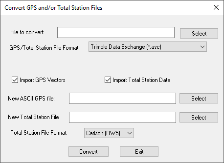
There is also a tool to convert Trimble Data Exchange total station data to either the Carlson RW5 format or the C&G CGR format. The following dialog box is displayed after choosing this option.
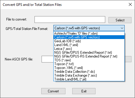
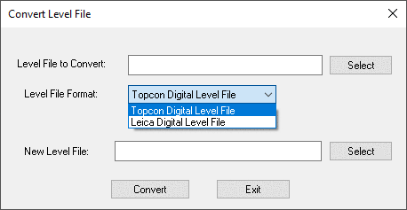
First choose the file format of the GPS vector file to be converted. Next use the 'Select' button to navigate to the vector file to be converted. If you are converting a Thales file you have the option to remove the leading 0's from Thales point numbers. Next, use the second 'Select' button to select the name of the new ASCII GPS vector file to be created. Choose the 'Convert' button to initiate the file conversion. Press the 'Cancel' button when you have completed the conversions. The file created will have an extension of .GPS. Following are examples of different GPS formats that can be converted to ASCII:
The purpose of this option is to convert differential level files from digital levels into C&G/Carlson differential level file format. At present the only level file format that can be converted are the level files downloaded from the Topcon digital levels.