Pressure_Pipe

This command models pressure pipe networks using methods and computations as required by the U. S. Environmental Protection Agency and compatible with EPANet software. This network, while using a .util file extension for data storage, is a separate model from utility or sewer networks. A pressure pipe network is made up of water source reservoirs, pumps, pipes, valves, water demand and storage tanks defined by horizontal and vertical alignment (centerline and profile), and parameters associated with the features of the network. The pressure pipe network models can be used in the Collisions Conflict Check command along with sewer and utility network models.

Clicking the Add button displays the Add Pipe dialog box prompting the user to select a Centerline file or to screen pick a polyline for a pipe. To add other entities, click the component heading, right-click to add. Add Pipe may also be accessed by right-clicking "Pipes" in the Pressure Pipe Network tree or by right-clicking on any existing pipe in the network.

Once the choice has been selected, the Edit Pipe dialog box appears. This box can also be accessed by clicking the Edit button or by right-clicking on an existing pipe in the network and choosing "Edit Pipe".

The Pipe Name is the name of the pressure pipe line. Each name must be unique in the pressure pipe network.

The Pipe Dim1 is the exterior diameter of the pipe. Carlson currently supports only round pipe in a pressure pipe network. When the size changes, use the Edit button to set the size at different stations along the line.

The Pipe Thickness is the thickness of the pipe's wall.

The Min Cover is the minimum depth for the pressure pipe profile. This value is used to create the profile and keep it below the reference surface. Also, the Report function has a report for checking the min cover.

The Roughness Coefficient is used to calculate friction loss in the pressure pipe network and is specific to the pipe material and the Analysis Method described below. Click the Set button to display a list of pipe materials with associated roughness coefficients.

The Plan View Linetype is used for drawing the pressure pipe line in the Draw Plan View function.

The Layer settings are used for drawing the pressure pipe line in the drawing.

The Profile Elevation Reference on Pipe controls the pipe position in the pressure pipe profile with respect to the reference surface and the Min Cover value.

The Centerline defines the horizontal alignment of the pressure pipe line.

The Profile defines the vertical alignment for the pressure pipe line.

The Edit Connections is an optional list of stations along the pressure pipe line where you can set a name, a 2-D drawing Symbol, a 3-D drawing Model, and a Demand for pressurized water at this Station.

The Insert button allows the user to enter a new Station, a name for the new Station, 2-D Symbol, 3-D Model, and water Demand at the new Station in volume per time.

The Delete button removes the currently highlighted connection from the Connection List.

The Edit Laterals is an optional list of stations along the pressure pipe line where Laterals are connected. A Lateral is defined by a Station, pipe size, Northing and Easting location of the Cleanout, Elevation of the Cleanout, and water Demand of the Lateral. Use the Pick button to screen pick the connection and cleanout points, or to pick an existing line for the lateral. The Connection and Cleanout Symbols are used for drawing the lateral in plan view.

The Insert button allows the user to enter a new lateral on the pipe being edited.

The Delete button removes a lateral from the pipe being edited.

The Edit Attributes button allows the assignation of attributes, previously defined on the Attributes tab in the Settings function, to the pipe. These Attributes are used in reporting.

The Remove button deletes the highlighted component from the pressure pipe network.

The Report button displays the Report dialog box.

The Data Files Report displays the files and parameters for each component of the pressure pipe network.

The Min Cover Check Report displays the Reference Surface and .util files used, and, for each pipe, the minimum cover as well as the average cover elevation.

The Quantities displays the Carlson Report Formatter, allowing the user to create custom reports using pressure pipe network information, import additional information, present the information in a variety of different formats, and export the report for other use.

The Output IFC File button creates a file that can be used by other software to import the 3-D model of the pressure pipe network.

The Pressure Pipe Network Settings button displays a multi-tabbed dialog box, defaulting to the "General" tab.

The Reference Surface is a triangulation file that is used for the min cover calculations and as a reference when editing pressure pipe profiles. The Auto Zoom to Current Selection check box finds and zooms to the component highlighted in the pressure pipe network tree. Highlight Current Centerline provides visual choices for in-drawing indication of the pressure pipe network component which has been selected.

On the "Plan View" tab, the Text and Symbol Size Scalers are used to set the size of pressure pipe network text and symbols for the Draw Plan View function. Clicking the "Set" button next to the Text Style field controls the font used for the pressure pipe network. The Label Name dropdown box allows the user to place the pressure pipe network component label at either end, at intervals defined in the Label Interval field, or choose "None" for no labels on components. Clicking the "Set" button beside The Pump, Tank, and Reservoir Symbols, selects the 2-D plan view symbols used for these components.

The "Color" tab sets the default colors to use when creating the layers used for drawing this and other Utility Networks.

On the "Attributes" tab, set any number of Attribute values or descriptions to associate with any components in the pressure pipe network. These can be displayed on the Quantities Report.

On the "Defaults" tab, the initial 2-D Connection Symbol and 3-D Connection Model are defined using the "Set" buttons. These may be changed when adding or editing a Connection.

Clicking the Draw button displays the Draw dialog box.

The 3D Polylines function creates a 3D polyline for each pressure pipe line. These polylines are tagged with their pipe size in the same format as the Assign Pipe Data to Polyline command.

The 3D Faces function draws each pressure pipe line as a 3D pipe using 3D faces. These 3D faces can then be used in the 3D Viewer commands.

The Plan View function draws a 2D polyline for each pressure pipe line and labels the line with its' name and connection points.

The Profile function displays the Select Profiles to Draw dialog box.

Set Reference Centerline allows the selection of a Centerline file to choose a Profile file. Add allows the selection of a Profile file. Add Multiple allows the selection of more than one Profile file choice at a time. Remove deletes a Profile from the list. Clear removes all Profiles from the list. Special Stations allows Station marks and elevation information to be displayed at other positions on the profile than at the beginning, end, and connection points by adding a new Station. Save Set saves the list of profiles to a user defined file name for recall. Open Set opens a previously saved Set. Multiple Profile allows the manipulation of Profile files containing more than one Profile.

To add a Pump, highlight the heading Pumps in the Pressure Network tree, right-click and select Add Pump. Highlighting an existing pump and right-clicking allows the choices Add Pump, Edit Pump, and Delete Pump.

When Add Pump is selected, the Add Pump Dialog Box is displayed, allowing the user to select a Centerline file or the selection an existing polyline on-screen.

Once this choice is made, the Edit Pump dialog box appears.

Name is the user defined name of the pump. Change the Centerline file by clicking the Centerline button. Clicking the Edit Button next to the Centerline file name allows the editing of the chosen Centerline file. The Start Elevation and End Elevation fields are used to set the pump's elevation in the system. These values are typically equal, but not necessarily. The Pump Parameters define the pump's operation by selecting a Keyword and assigning
a Value or a Curve. None assigns no parameters to a pump. A pump must be either a Power pump or a Head pump. Power illuminates the Value field where a constant energy in Kilo-Watts is entered, reporting the same energy requirement for any combination of water volume and pressure. Head illuminates the Curve field. A pump Curve plots the relationship between flow volume and head. Curves can be created or edited using the Edit Curve button or the Edit button in the Keyword area prior to assigning it to a pump. If Head is selected, either the Speed or Pattern keyword may also be selected. Speed modifies the pump speed, which is assumed to be 1, shifting the position of the Head pump curve by speeding up the pump with a value greater than 1, decreasing the pump speed with a value less than 1 or shutting the pump off with a value of zero. Pattern allows the selection of a pattern number which allows variable pump speeds through time. Once a Keyword and Value are entered, click Add to save the parameter. Highlight the Keyword and click Delete to remove the parameter.

To add a Reservoir, highlight the Reservoirs heading in the Pressure Pipe Network tree, right-click and select Add Reservoir. Highlighting an existing Reservoir and right-clicking allows the choices of Add Reservoir, Edit Reservoir, or Remove Reservoir.

When Add Reservoir is selected, the Add Reservoir Dialog Box is displayed.

Select the Reservoir location by clicking the arrow in the dropdown box next to "Pipe". Reservoirs may also be connected to pumps. A pump may be connected to only one reservoir and will disappear from the pipe and pump list if already assigned to a reservoir. Select whether the reservoir is at the Start or End of the pipe or pump. Name the reservoir. Set the elevation of the Hydraulic Head.

To edit a reservoir, select an existing reservoir name, right click and choose Edit Reservoir, causing the Edit Reservoir dialog box to appear.

Change values as needed, click OK to save changes.

To add a Tank, highlight the Tanks heading in the Pressure Pipe Network tree, right-click and select Add Tank. Highlighting an existing Reservoir and right-clicking allows the choices of Add Tank, Edit Tank, or Remove Tank.

When Add Tank is selected, the Add Tank Dialog Box is displayed.

Clicking the arrow in the dropdown box beside Pipe allows the selection of the component the tank attaches to. Start and End buttons are used to set the tank's location with respect to the component. Name the tank. The Bottom Elevation is the tank's minimum gravity head, the bottom of an empty tank. Initial Water Level is the starting water level elevation of the analysis. The Minimum Water Level is the least amount of water desired in the tank entered as an elevation. Maximum Water Level is the maximum amount of water desired in the tank entered as an elevation. Nominal Diameter is the average cross-sectional area of the tank used to convert a change in water volume to the change in water level elevation in the tank. The Minimum Volume is the least amount of water allowed in the tank which should be equivalent to the Minimum Water Level. In the future, you will be able to assign a Volume Curve to the tank to model tanks of different shapes with cross-sections that vary by elevation.

To edit a reservoir, select an existing reservoir name, right click and choose Edit Tank, causing the Edit Tank dialog box to appear.

Change values as needed, click OK to save changes.

To add a Valve, highlight the Valves heading in the Pressure Pipe Network tree, right-click and select Add Valve. Highlighting an existing Reservoir and right-clicking allows the choices of Add Valve, Edit Valve, or Remove Valve.

When Add Valve is selected, the Add Valve Dialog Box is displayed, allowing the selection of a Centerline file or the selection of an existing polyline on-screen.

After selection, the Edit Valve dialog box appears.

Name the Valve. Clicking the Centerline button allows a choice of a new Centerline file. Clicking the Edit button here allows the editing of the Centerline. Enter the Start Elevation and End Elevation. Assign a valve Type.
A Pressure Reducing Valve, Pressure Sustaining Valve, or Pressure Breaker Valve require a Setting pressure. A Flow Control Valve requires a Setting of limiting volume. A Throttle Control Valve requires a Setting of a loss coefficent supplied by the manufacturer of the valve. A General Purpose Valve requires the application of a Headloss Curve. A Diameter in inches or mm of the valve is required for all valves. A Loss Coefficient may be applied to any valve or may be zero.

Selecting the EPANet button displays EPANet dialog box and defaults to the "Hydraulics" tab.

The Analysis Method dropdown box allows the selection of one of three methods supported by EPANet.

The Units dropdown box allows the selection of the desired volume per time unit.

The "Times" tab allows setting parameters for either a single time period or an extended analysis.

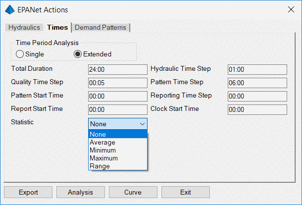
If Time Period Analysis - Single is selected, all other fields on the tab are deactivated, setting up a "snapshot" analysis of the pressure pipe network.

If Time Period Analysis - Extended is selected, all fields on the tab are available for edit. Total Duration is the total length of time to be analyzed. Water quality is not currently being analyzed in Carlson 2019. Quality Time Step is not currently used. Pattern Start Time is the time the Demand Patterns created and listed on the "Demand Patterns" tab starts. Report Start Time is the first time shown on the analysis. Hydraulic Time Step is the time unit incremented as the analysis proceeds through the Total Duration. Pattern Time Step is the time unit used to step from one Demand Pattern to the next. Reporting Step Time defaults to the Hydraulic Time Step unless and different increment is assigned in this field. Clock Start Time is when the analysis begins. The Statistic controls how information is presented in the Analysis report. None reports data at each Reporting Time Step increment or, if zero, the Hydraulic Time Step. Average reports the average values found for the Total Duration. Minimum reports the minimum value, Maximum reports the maximum value and Range reports minimum and maximum values across the Total Duration.

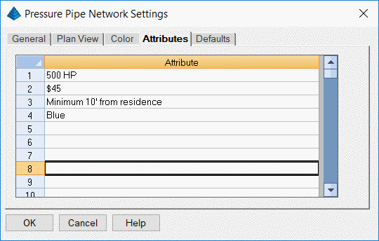
The "Demand Patterns" tab allows the weighting of water demand assigned to connections and laterals when creating the pressure pipe network based on time of day.

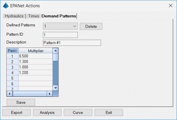
Select an existing pattern to be used to weight the demand during different times of the day. To add a new Pattern, type a new Pattern ID, a new Description, desired Multipliers and click Save.

In the example above, the Clock and the Pattern start at midnight and the demand is reduced by the Multiplier 0.50 until the Pattern Time Step increment comes due at 6am, increasing the demand by 1.3. At noon, demand drops to its' default values, then at 6pm demand is increased by a factor of 1.20. Note that the Pattern Time Step and the number of Multipliers are synchronized.

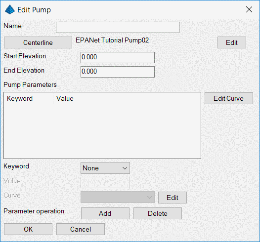
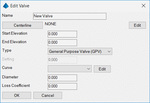
Next, develop a pump curve by clicking the Curve button. By specifying the Type, the values in the X and Y columns are defined.

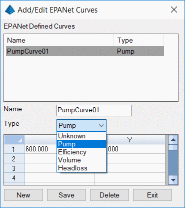
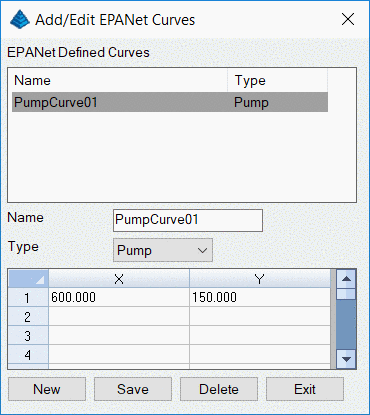
The Curve Type Pump develops a single-point or multi-point Pump Curve plotting volume per unit time (flow rate) in the X column, head in the Y column. An Efficiency Curve plots a pump's flow rate in the X column vs. energy use efficiency as a percentage in the Y column. A Volume Curve plots flow rate in the X column vs. the change in elevation (head) in a tank and is used to model tanks with non-uniform cross sections. A Headloss Curve plots the flow rate in the X column vs. the headloss in feet or meters in the Y column as water flows through a General Purpose Valve.

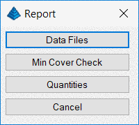
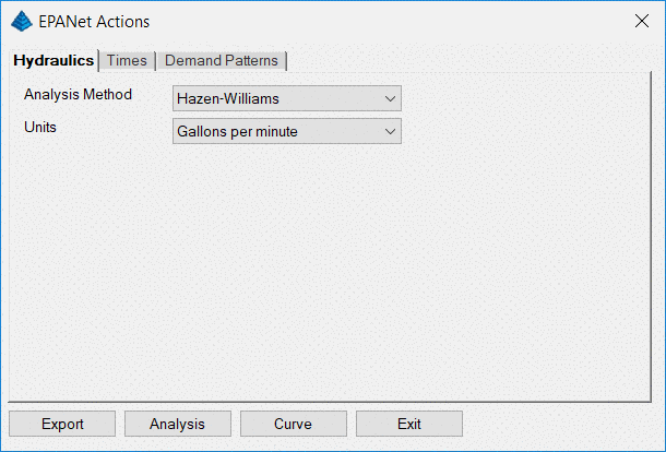
The Analysis button produces a report that can be viewed, saved, printed and search showing demands, flow rates, head, energy consumption, pressures, velocities and headlosses in the Network, either as a snapshot or with a Demand Pattern applied.

The Export button creates a file which can be imported into EPANet.

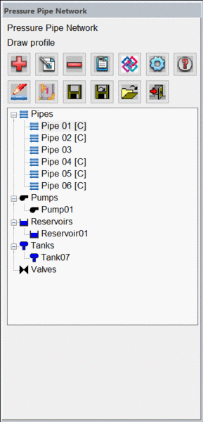
Pulldown Menu Location: Network
Keyboard Command: epanet
Prerequisites: Centerline files, Profile files and/or polylines representing pipes, pumps, and valves.