Prepare Value Block Model
This command creates a block model that represents
the economic value of each block. The value block model can be
generated from multiple .blk files, a Geologic Model (.pre file),
or from an existing .BM file. The blocks loaded into this command
can be modified with user-defined equations to determine the value
of each block. The value block model may then be used with the
Optimized Pit Design command.
When the command is first executed, the below
dialog will appear.
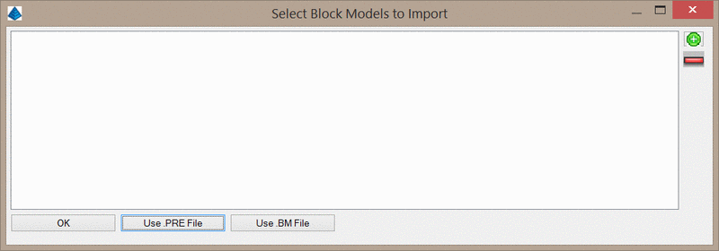
To load in .blk files, you can simply add/remove them by using the
green plus icon and the red minus icon on the right of the dialog.
There should be no gaps between the elevation limits of these block
models. The ordering of these files is not important, as they will
be sorted automatically according to the elevation limits of each
.blk file.
The Use .PRE File button will prompt you to select a .pre
file to generate the blocks. This option will convert a stratified
Geologic Model into a single block model by specifying a number of
vertical divisions to apply to each strata/bed. When this button is
clicked, the below dialog will appear.
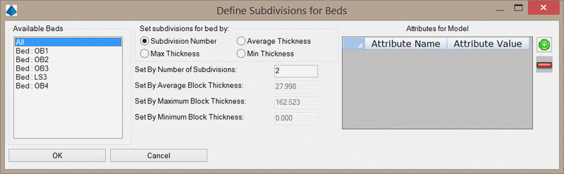
Available Beds: This column will list all of the
strata/beds in the .pre file that are not already defined with a
.blk file. Selecting one of these beds will allow you to define the
subdivisions for that bed. Alternatively, you may set the
subdivisions for all beds at once.
Set Subdivisions for bed by: This option control how each
bed will be vertically subdivided to create a block model.
Subdivision Number: This option will subdivide
the bed by the number specified. For example, if this value is set
to 2, then the resulting block model of the bed will consist of 3
blocks per vertical column. Note that this value must be greater
than or equal to 2.
Set By Average Block Thickness: This option will set the
number of subdivisions in order to achieve the specified average
block thickness. For example, if this value is set to 10, the bed
will be subdivided so that the average block thickness of the
resulting model will be as close to 10 as possible.
Set By Maximum Block Thickness: This option will set the
number of subdivisions in order to achieve the specified maximum
block thickness. For example, if this value is set to 10, then the
bed will be subdivided so that no blocks in the resulting model
have a thickness greater than 10.
Set By Minimum Block Thickness: This option will set the
number of subdivisions in order to achieve the specified minimum
block thickness. For example, if this value is set to 10, then the
bed will be subdivided so that no blocks in the resulting model
have a thickness less than 10.
Attributes for Model: This spreadsheet allows you to define
new attributes to add to each block in the model. These attributes
can will be set to single values, but can be modified when
calculating the value of each block. At least one attribute must be
defined for each bed.
The Use .BM File button will prompt you to select an
existing .BM file. Note that .BM files are exported from this
command.
After selecting one of these options, the below dialog will
appear.
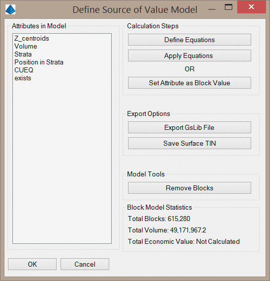
Any attributes from the input files will be listed on the left
side of the dialog. These attributes may be used when writing
equations to define the value of each block. Note that when these
attributes are referenced, it refers to the value of each block
individually - these are not average values for the block model as
a whole. In addition to the attributes from input, four additional
attributes will always be generated: Z_centroids and
Volume.
The Z_centroid attribute is the elevation of each block's
centroid.
The Volume attribute is the volume of each block, as measured in
cubic feet/meters.
The Strata attribute is the strata index number. A value of 0
relates to the upper-most strata in the model, a value of 1 relates
to the strata below strata 0, etc.
The Position in Strata attribute is the block number counted from
the bottom of the model. For example, the lowest block in the bed
will be block 1, the next block up will be block 2, etc.
Define Equations: This button will allow you to create an
equation file (.db3 file). Additional information about this
function is provided below.
Apply Equations: This button will calculate the value
block model according to an equation file (.db3 file). Note that
this button does not modify the input files - you will be prompted
to save the updated model as a .BM file after clicking
OK.
Set Attribute as Value: This button will set the currently
selected attribute as the economic value for each block in the
value block model. This is an alternative to calculating the block
values from a set of equations. Note that this button does not
modify the input files - you will be prompted to save the updated
model as a .BM file after clicking OK.
Export GsLib File: This button will export the value block
model to a .txt file in a GsLib format.
Save Surface TIN: This button will create a .tin file of
the surface of the value block model. Note that this surface will
have a block-like appearance and will therefore differ from the
original upper limit of the input .blk files.
Remove Blocks: This button will prompt you to select a an
elevation.grd file. You will then be prompted to if you would like
to remove blocks found above/below this elevation grid.
Block Model Statistics: These values display basic
information about the value block model.
Total Blocks: The total number of blocks in the
value block model. Null blocks are not considered in this
counter.
Total Volume: The sum of the volume of all blocks in the
model.
Total Economic Value: The sum of the economic value of all
blocks in the model. This value will not be populated until the
equations have been applied to the blocks or until an attribute has
been set as the block economic value.
Define Equations Dialog
After clicking the Define Equations button, the below dialog
will appear. After saving this table to a .db3 file, you may return
to the previous dialog to calculate the value block model.
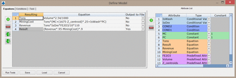
The dialog will first appear with only one Equation and
Predefined attributes. All other equations, constants, conditions,
etc. must be manually added.
Attribute List
The right side of the dialog lists all attributes. You can add
or remove attributes with the two icons shown to the left of the
list. Attributes may be one of five types, with each type showing
with a unique color for visual organization.
- Predefined attributes are attributes that have been found in
the input .blk file(s).
- Equations are attributes that will be calculated when the value
block model is created.
- Constants are attributes that have a non-changing
value.
- Conditions are logical tests that determine which variables to
use. For example, you may define a condition that sets the
processing cost for a block based on grade.
- Conditional Variables are used as a result when Conditions are
checked. For example, when setting the processing cost of a block
based on grade, the processing cost is the Conditional
Variable.
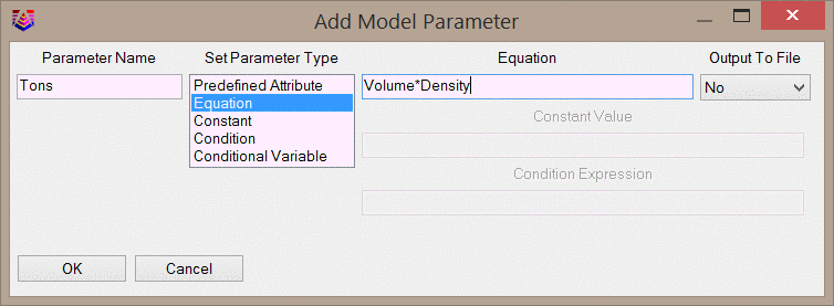
When adding an attribute, the below dialog will appear. Here you
can give the attribute a name and set the attribute type. You may
also set any other relevant options for the selected attribute
type.
Attributes may be renamed by clicking inside the cell of
interest and typing a new name. When the name of an attribute is
modified, the change will be reflected in the Equations and
Conditions tabs on the left side of the dialog. You may also change
the condition type by selecting an option from the pulldown menu in
the Type column.
Equations Tab
The Equations tab will display all defined equations in a
spreadsheet view.
The Resulting Attribute column lists the attribute being
calculated by the Equation column. For example, if you have a
Resulting Attribute named "Tons", the result of the equation column
will be assigned to this "Tons" attribute.
The Equation column is where you will write the equation for the
attribute being calculated. For example, if you are calculating the
"Tons" for each block, the equation could simply read
"Volume*Density". This can be read as "Tons equals Volume
multiplied by Density", where Volume and Density are other defined
attributes. Equations will be calculated in from top to bottom by
row, and therefore equations may reference the results from
previously calculated equations. For example, the equation on the
row 2 of the equation spreadsheet may reference the result from row
1, but it cannot reference the result from row 3.
The Output to File column controls if the attribute is output to
the resulting .bm file. By default, attributes will not be saved to
the .bm file. If the .bm file is to be used with the Optimized Pit
Design command, only the economic value of each block should be
output to the .bm file.
One equation, "Result", will always be defined and output to the
.bm file. This equation should always define the value of each
block and should always be output to the .bm file.
The below operations and the corresponding symbol are supported
in the equation column:
- Addition "+"
- Subtraction "-"
- Multiplication "*"
- Division "/"
- Grouping of terms "(" and ")"
Conditions Tab
The conditions tab will display all conditions in a spreadsheet
view as shown below.
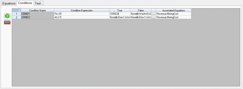
The Condition Name column lists the conditions in the order they
were created. These cells are not editable.
The Condition Expression column is the logical test. In the
above example, the first logical test checks if the block has an
Iron content greater than 20%.
The True column lists the actions to take if the logical test is
found to be true. At least two actions will be shown, separated by
a vertical pipe. The first action tells the program which condition
to evaluate next. The second action actually sets values to the
Conditional Variables. In the above example, if a block is found to
have an Iron content greater than 20%, the program will check
Condition #2, but no Conditional Variable values will be assigned
based on this test alone. If Condition #2 is found to be true, the
program will not check another condition, but will assign the
attributes "IsWash" and "IsOre" values of 1. This is similar to a
nested "if" statement.
The False column lists the action to take if the condition is
found to be false. This follows the same format as the True column.
In the above example, if a block is found to have an iron content
less than or equal to 20%, then no other condition is evaluated and
the "IsWash" and "IsOre" conditional variables are assigned a value
of 0.
If you click inside a cell of the True or False columns, the
below dialog will appear.
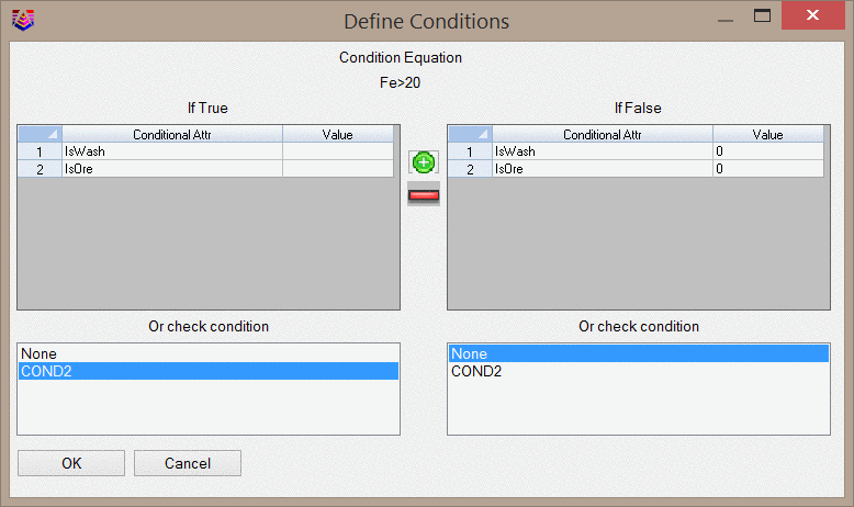
This dialog sets values for the Conditional Variables based on
the logic of the Condition. The two tables list Conditional
Variables that will be affected by this Condition (IsWash and IsOre
in this case). If the program needs to check another Condition
rather than assign values to Conditional Variables as a result of
this test, you may select the appropriate Condition to check below
this Table. Conditional Variables may be added/removed from this
list using the appropriate icons between the two tables.
The Associated Equations column lists the equations in which the
conditions need to be evaluated. In the above example, both
conditions will be evaluated when the Revenue and MiningCost
equations are calculated.
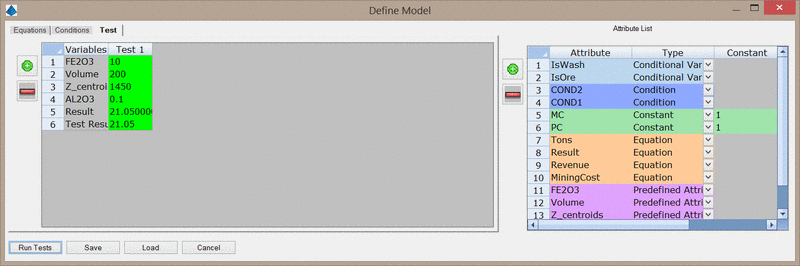
Test Tab
The Test tab displays all defined attributes in a simple
spreadsheet. The purpose of this tab is to define example values
for each attribute, along with an expected result. After defining
one or more tests and saving the .db3 file, you may click the
Run Tests button to check the actual output against the
expected output. If the Test Result matches the expected result,
the cells will be highlighted in green, as shown below. If the
values do not match, the cells will be highlighted in red.
Keyboard Command:
mkvalblkm
Pull-down Menu Location:
Geology Module > Block
Model
Prerequisite: Must have an
existing BLK file