Haul Cycle Analysis
This command is used for detailed analysis of haul routes using
various haul trucks to determine either 1) the required truck fleet
required to meet a target production or 2) the attainable
production based on a given haul fleet. This command requires the
user to have executed the Haul Road Manager to define the haulage
route. Although optional, it is recommended to define and customize
truck parameters using the Haul Fleet Manager command to ensure the
most accurate results. The first section of this document discusses
the basic use of this routine, while the second section discusses
the actual calculations that are performed to analyze the haul
cycle.
Basic Use
First, you will be prompted to select the start and ending points
of the haul road to be considered. The dialog that appears will
show a spreadsheet view of all potential routes between the
starting and ending point which will be sorted by distance in
increasing order. The dialog will change slightly depending on the
‘Calculate’ option selected (either Fleet Size or Production).
- Preview Window: highlights the currently selected haul
route. This window works very similar to the 3D Viewer Window.
Using the four icons next to this screen, you can pan, zoom,
rotate, and zoom to the extents of the haul route.
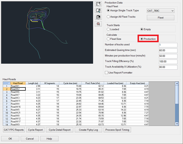
- Production Data Section: allows you to choose the type
and amount of haul trucks to be used for the cycle analysis. The
‘Assign Single Truck Type’ option will allow you select one of the
trucks defined in the Haul Fleet Manager library. The ‘Assign All
Fleet Trucks’ option will use the types and amounts of trucks
defined in the same library. Clicking the ‘Fleet’ button will allow
you to edit this library. Using the ‘Assign All Fleet Trucks’
option will only allow you calculate the attainable production
rate. For more information on the Haul Fleet Manager, see the
appropriate section of the help manual.
- Truck Starts option: allows you to specify if the
selected starting point represents the loading or the dumping point
of the route.
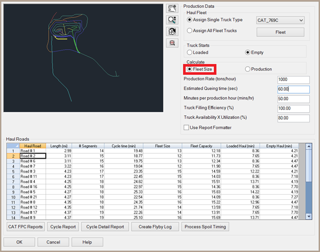
- Calculate option: changes the routine to calculate
either the required fleet size based on a production target, or the
attainable production target based on the haul fleet.
- Production Rate: This value can be set when calculating
the required fleet size. This sets the target production the haul
fleet must meet.
- Number of trucks used: This value can be set when
calculating the attainable production when using the ‘Assign Single
Truck Type’ option.
- Estimated Queuing time: This the estimated time that the
truck must wait in line at either the loading or the dumping point
per cycle (25 second wait at the loading point and 15 seconds at
the dumping point would be a total Estimated Queuing time of 40
seconds).
- Minutes per production hour: This is the expected
working time per hour. This is essentially a measure of work
efficiency, and should therefore account for variable delays due to
factors such as:
-
- Excavating equipment delays
- Personnel delays
- Climate delays
- Truck Filling Efficiency: This is the fill percentage of
the truck. A 90% filling efficiency applied to a truck that is
intended to carry 100 tons will only carry 90 tons per cycle.
- Truck Availability X Utilization: This value is
multiplied by the Minutes per Production Hour to determine the
total working time of the truck. It is intended to account for
fixed delays and mechanical availability of the truck. For a truck
listed as working 50 minutes per production hour, an Availability X
Utilization value of 90% will result in only 45 working minutes per
hour.
- Use Report Formatter: This option will allow you use the
Report Formatter for the Cycle Report and the Cycle Detail Report
to customize the reported information.
Reports
The Haul Cycle Analysis command is very quick and dynamic. Whenever
a value is edited, the results in the spread sheet view will be
automatically updated. These results can be reported in a variety
of formats as discussed below.
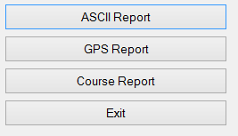
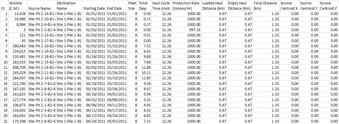
CAT FPC Reports: This option will allow you to export one of
three report types: ASCII, GPS, and Course.
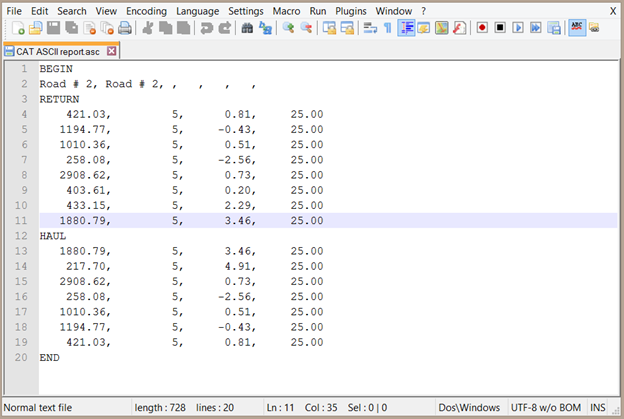
The ASCII report will export the segment distance, the rolling
resistance, the slope, and the speed of the truck along each
segment into an .asc file as shown below:
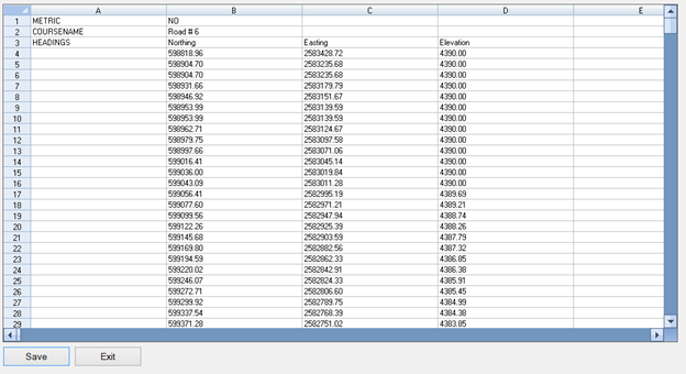
The GPS report will export the coordinates and elevation of the
haul road at each vertex representing the road. This report can be
saved as an Excel spreadsheet (.xls file) as shown below:
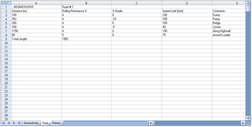
The Course Report is reported in a spreadsheet with three tabs:
General Info, Haul, and Return. This file can also be saved as an
Excel spreadsheet, as shown below:
Cycle Report: This report gives basic information about the
haul cycle.
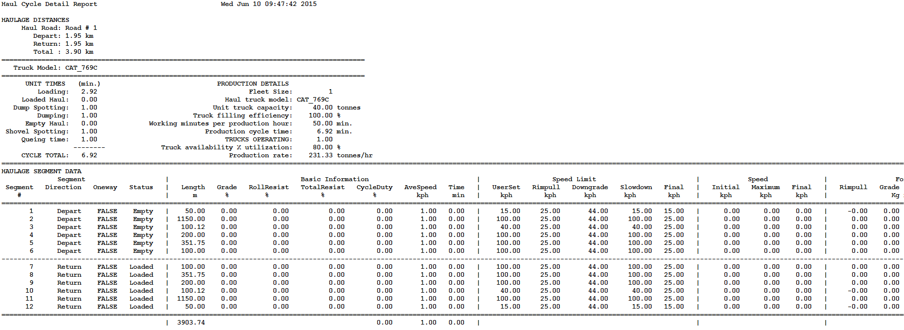
Cycle Detail Report: This report provides more detailed
information about the haul cycle, which in addition to the
information in the standard report, provides information about the
transition of speed along each segment, the rimpull applied on each
road, and detailed information about the sub-segments which are
used in the calculations.
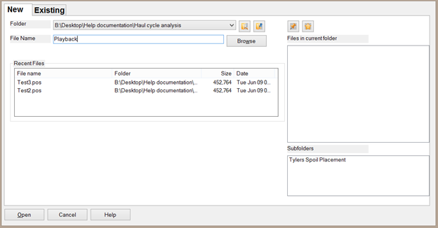
Create Flyby Log: This option will create a .pos file which
can be reviewed with the Surface 3D Flyover command in the Civil
module. You will be prompted to enter a road width, then you will
be allowed to specify the file name.
Process Spoil Timing: This command will perform a timing
analysis on an exported .sph file from Spoil Placement Timing. This
will give a more detailed analysis of the haul cycle during each
time period of the spoil placement. An example report is provided
below:
Calculation Methods
A good planner will be cautious about blindly accepting
calculations. For this reason, the following section details the
logic and calculations used in Haul Cycle Analysis so that the user
can fully understand how the routine works.
As previously stated, this routine seeks to calculate either the
attainable production based on the truck fleet or the fleet size
required to meet a target production. Actually determining these
values is rather simple once to the true cycle time has been
calculated. However, calculation of the cycle time considers many
factors. The first sub-section of this section details how the
program calculates cycle time. The following sub-section details
how the attainable production and required fleet size are
calculated based on the calculated cycle time.
Calculation of Cycle Time
The diagram shown below is visual outline of the equations used to
calculate the haul cycle time. This is provided to allow for a
better understanding of how Haul Cycle Analysis uses input
variables to determine various operating parameters. Note that this
diagram is simplified, and does not detail all of the logic used in
the actual routine.
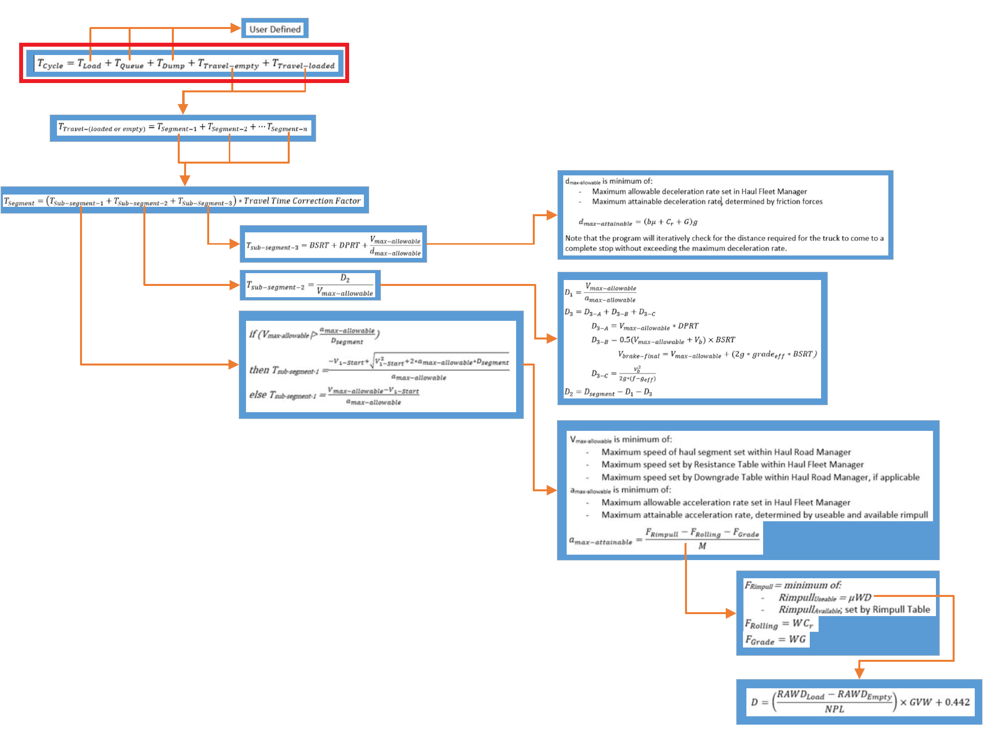
The total haul cycle time can be calculated with the following
equation:
 where
where
- TCycle is the total cycle
time
- TLoad is the time required to
load the truck
- TTravel-loaded is the time
required for the truck to travel from the loading point to the
dumping point
- TQueue is the total estimated
queuing time (sum of queuing time at both the loading point and the
dumping point)
- TDump is the time required
for the truck to dump its payload
- TTravel-empty is the time
required for the truck to return to the loading point from the
dumping point
Three variables, TLoad, TDump, and
TQueue, are manually entered. The remaining
variables, TTravel-loaded and
TTravel-empty, are calculated similarly to one
another, but with different values based on the road profile and
truck specifications for loaded and empty scenarios.
TTravel-loaded and TTravel-empty are
calculated with the following formula:
TTravel-(loaded or
empty)=TSegment-1+TSegment-2+⋯TSegment-n
where
TSegment-1 is the travel time of
the first segment of the haul route
TSegment-2 is the travel time of
the second segment of the haul route
Etc.
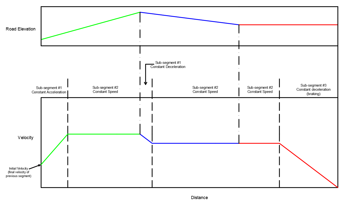
The travel time for a single haul segment will be further divided
into three sub-segments according to the following chart.
Sub-segment #1: the truck is
accelerating/decelerating at a constant rate
Sub-segment #2: the truck is traveling at
a constant velocity
Sub-segment #3: the truck is braking.
Note that sub-segment #3 is only used when the truck comes to a
complete stop.
In the below picture:
- The top portion of colored lines represent
the road profile, broken into three haul segments
- The lower portion of colored lines represent
the velocity of the truck along the haul road
- Haul Segment 1 (green line)
- Sub-segment #1 shows the truck accelerating
as it travels uphill to meet the new road speed limit
- Sub-segment #2 shows the truck traveling at
a constant velocity once it reaches the road speed limit
- Haul Segment 2 (blue line)
- Sub-segment #1 shows the truck decelerating
as it starts to travel downhill to meet the new road speed
limit
- Sub-segment #2 shows the truck traveling at
a constant velocity once it reaches the road speed limit
- Haul Segment 3 (red line)
- Sub-segment #2 shows the truck traveling at
a constant velocity. It is traveling at the speed limit when it
approaches Haul Segment 3.
- Sub-segment #3 shows the truck braking as
the truck comes to a complete stop.
The total travel time for a haul segment is simply a sum of the
sub-segment travel times, as shown below:
TSegment=(TSub-segment-1+TSub-segment-2+TSub-Segment-3)
The travel time of each sub-segment is calculated using the
following formulae:
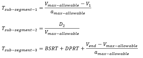
where
- TSub-segment-1 is the travel
time of sub-segment #1
- Vmax-allowable is the maximum
allowable truck velocity along the haul segment
- V1-Start is the truck
velocity at the start of sub-segment #1, equal to zero at the
beginning of the haul route
- amax-allowable is the maximum
allowable acceleration of the truck on sub-segment #1
- TSub-segment-2 is the travel
time of sub-segment #2
- D2 is the distance of sub-segment #2
- TSub-segment-3 is the travel
time of sub-segment #3
- BSRT is the Brake System Response Time
- DPRT is the Driver Perception Response
Time
- dmax-allowable is the maximum
allowable deceleration rate of the truck
Sub-Segment #1 Supplement
Vmax-allowable is minimum
of:
- Maximum speed of haul segment set within
Haul Road Manager
- Maximum speed set by Resistance Table within
Haul Fleet Manager
- Maximum speed set by Downgrade Table within
Haul Road Manager, if applicable
amax-allowable is minimum
of:
- Maximum allowable acceleration rate set in
Haul Fleet Manager
- Maximum attainable acceleration rate,
determined by useable and available rimpull
Note that a truck’s velocity does not necessarily have to increase
during sub-segment #1. If a truck enters a haul segment at a speed
which exceeds the maximum allowable velocity for the haul segment,
then sub-segment #1 will refer to a decelerating situation.
Sub-Segment #2 Supplement
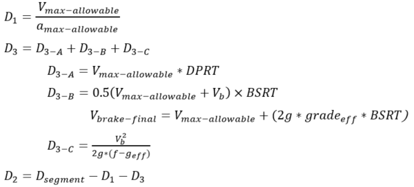
In the final report, sub-segment distances will be reported as D1,
D2, and D3, which refer to the distances of the respective
sub-segments. The distance for each sub-segment is calculated as
shown below. Here it is also important to note that the sub-segment
#3 is further divided into three sections which represent A) the
time required for the driver to realize that a stop is required, B)
the time from when the driver first applies the brake to the time
when the brake system applies the full braking force, and C) the
time required for the truck to stop once the full braking force is
applied.
Note that in many situations one or two of these sub-segments will
not be used in the final calculations. For example, if a truck
enters a new haul segment and does not need to
accelerate/decelerate to meet the speed limit, the distance and
travel time for sub-segments #1 and #3 will be zero. As another
example, sub-segment #3 will only be used when the truck is braking
to a complete stop.
where
- D1 is the distance of
sub-segment #1
- D2 is the distance of
sub-segment #2
- D3 is the distance of
sub-segment #3
- D3-A is the distance of
sub-segment #3, section A
- D3-B is the distance of
sub-segment #3, section B
- D3-C is the distance of
sub-segment #3, section C
- DSegment is the length of the
current haul segment
- Vb is the truck velocity at
the end of the Brake System Response Time
- g is the acceleration due to gravity
- f is the coefficient of friction available
for braking (
- geff is the effective grade,
which is a sum of the road grade and the rolling resistance of the
road on the tires
Sub-segment #3 Supplement
dmax-allowable is minimum
of:
- Maximum allowable deceleration rate set in
Haul Fleet Manager
- Maximum attainable deceleration rate,
determined by friction forces
Note that the program will iteratively check for the distance
required for the truck to come to a complete stop without exceeding
the maximum deceleration rate.
Max Truck Acceleration/Deceleration
Both sub-segments #1 and #3 must check for the maximum allowable
acceleration/deceleration rate, and one of the rates to be
considered is the rate limited by friction, also referred to as the
useable rimpull. The below equations show how the
acceleration/deceleration rates are calculated.
As previously shown, Haul Cycle Analysis analyzes truck movement by
constant acceleration/deceleration along sub-segments and sections
of sub-segments. For this reason, the acceleration of the truck can
be defined by scalar quantities in Newton’s Second Law of motion,
shown below and simplified:
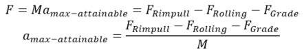
where
F is the sum of all forces acting on the
truck
M is the mass of the truck
amax-attainable is the maximum
possible acceleration of the truck
FRimpull is the effective rimpull
force (minimum of available rimpull and useable rimpull force)
FRolling is the force of rolling
resistance, which is set within the Haul Road Manager for each haul
segment
FGrade is the grade resistance
force, defined as positive for uphill and negative for downhill
movement
FRimpull
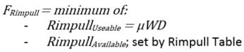
Available Rimpull is determined from standard Rimpull Curves
provided by truck manufacturers. This data is entered into the Haul
Fleet Manager in a tabular format in the Rimpull Table. From the
entered values, the program will determine the available rimpull at
various operating speeds.
Useable rimpull is the maximum force the truck can apply before the
tires start to slip on the road. This value is calculated with the
following equation
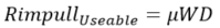
where
- RimpullUseable is the useable
rimpull force
- μ is the traction coefficient between the
road and the tires, which is set in the Haul Fleet Manager
- W is the truck weight
- D is the ratio of the truck weight on the
rear axle
Furthermore, D can be calculated with the following equation
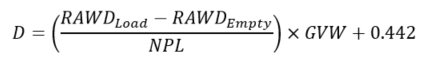
where
RAWDLoad – drive (rear) axle
weight distribution percentage in loaded condition, expressed as a
decimal
RAWDEmpty – drive (rear) axle
weight distribution percentage in empty condition, expressed as a
decimal
NPL – nominal payload
GVW – gross vehicle weight; note that will not
always equal the loaded truck weight
FRolling
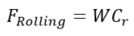
Where
Cr is the haul segment rolling resistance, expressed
as a decimal; this is set in the Haul Road Manager
FGrade
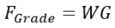
Although this calculation does not perfectly calculate the
resistive/assistive force due to the grade of the road, the
difference between the calculated value and the ‘true’ value is
considered insignificant. Once the maximum possible acceleration of
the truck has been calculated, this value is compared to the
maximum acceleration limit set in the Haul Fleet Manager. The
minimum of these two values is used for the calculation of the
distance and travel time of sub-segment #1 for each haul
segment.
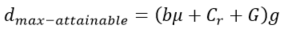
Maximum Deceleration
When a truck slows down, it is limited to using the lesser of two
possible deceleration rates. One rate is defined directly in the
Haul Fleet Manager. The other rate is calculated based on Newton’s
Second Law using the below formulae:

where
- FAvailable is the total
available retarding force
- dmax-attainable is the
maximum attainable retarding deceleration rate
- M is the mass of the truck
- FRetard is the retarding
force
- FRolling is the rolling
resistance force
- FGrade is the grade
resistance force
- b is the braking reliance on traction
- μ is the traction coefficient
- Cr is the rolling resistance
coefficient
- G is the road grade; uphill is positive,
downhill is negative
- g is the acceleration due to gravity
- W is the truck weight
Calculation of Required Fleet Size and Attainable
Production
Once the total cycle time has been calculated, the calculation of
the required fleet size/attainable production is very simple. The
calculations for these values are shown below
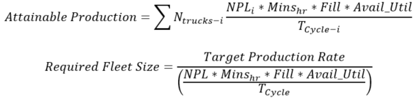
Where
- NTrucks-i is the number of
trucks of a specific model
- NPLi is the nominal payload
of a specific truck model
- Minshr is the minutes working
per production hour
- Fill is the truck filling efficiency
- Avail_Util is the truck availability
multiplied by the truck utilization
- TCycle-i is the truck cycle
time for a specific truck model
Note that the total attainable production is the sum of each
attainable production rate of each truck in the haul fleet.
References:
Parreira, Julianna. "An Interactive Simulation Model to Compare an
Autonomous Haulage Truck System with a Manually-Operated System."
Diss. THE UNIVERSITY OF BRITISH COLUMBIA (VANCOUVER), 2013.
Print.
U.S. Department of Labor. MSHA Haul Road Inspection Handbook. June
1999. Handbook Number PH99-I-4.
Prompts
Delay: Intersection
Merge (will be a pre-named delay name)
[near on] Pick start point on Haul Road: select where the
truck will begin, usually where it gets loaded at.
[near on] Pick end point on Haul Road: select where the
truck will end, usually where it unloads/dumps at.
Pull-Down Menu Location: Reserves/Timing in
Surface Mining
Keyboard Command: haul_cycle