This lesson will step through modeling a limestone quarry using
the Carlson block model routines. It goes through the process from
start to finish, importing drillholes to final reporting and
viewing graphics. Most of these commands are found in the Block
Model menu of the Carlson Geology Module.
Step 1—Import the
Drillhole and Face Data
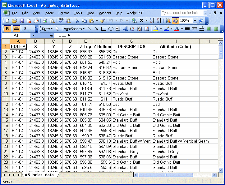
To import the drillhole data, it is important to create an ASCII
file with a repetitive series of columns for the collar x,y,z
position, followed by columns for the downhole information. Shown
here is an example of the spreadsheet to import.
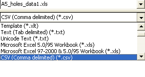
To import the drillholes, it will need to be in ASCII form, use Excel to save the file in ASCII form with a “.csv” extension.
Answer Y to the question regarding saving the current worksheet. This results in a comma-separated file ASCII, such as this typical example, viewed with Notepad:
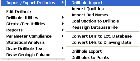
Notice that this file contains one “header” line consisting of the title, that we can ignore. Next we bring this file into Carlson by using the command Drillhole Import found in the Import/Export Drillhole flyout, underneath the Drillhole pulldown menu.
Before selecting this command, it is a good idea to pre-set the
drillhole symbol to be used within the command Define Drillhole,
located in the same Drillhole pulldown menu. Note that there is a
rather large 25-unit drillhole dimension and have chosen a solid
circle symbol, to distinguish the drillholes from the face data
(which will use a small, solid square symbol). Also make sure the
default Density is set for the ore.

By choosing “Save” in the lower left of the dialog, these settings are saved in the CH file named earlier. Then with the command Drillhole Import, the CH file will set the default symbol format. Now choose Drillhole Import and within this command, choose the Custom Import Formatter.
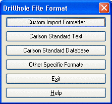
This window will appear:
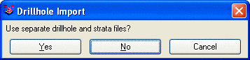
Note that the default answer is “No” and can be selected by pressing Enter. Load the correct “.csv” file containing the ASCII drillhole data. Now organize the right-hand column to correspond to the ASCII file, as shown here:
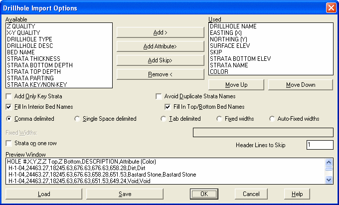
Note how you can study the data file organization in the “Preview Window”. This format can be given a name and saved by pressing the Save button. Note that we have specified “1” header line to skip (skip the title line) at the bottom right of the dialog, and also notice that we have chosen to skip the “Z Top” column, since the bottom elevation defines the strata, measuring down from the top, collar elevation. Press OK to continue. As a result of the import, we now have 7 drillholes in our area of study, as shown below:

Importing Drillholes is a critical process in geologic modeling, so it is important to be familiar with the precise techniques to accomplish this. Carlson offers extremely flexible importing. The drawing with the 7 new drillholes can now be saved with any file name desired.
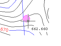
You have the option to import these drillholes while already in a drawing (such as a topo map of the site), or you can import the drillholes into a blank drawing then insert additional surface features like contours. The Insert command can be found under the Draw pulldown in Carlson. In this case, we’ll insert a contour file called Block Model Contours, to obtain the combined drawing below:
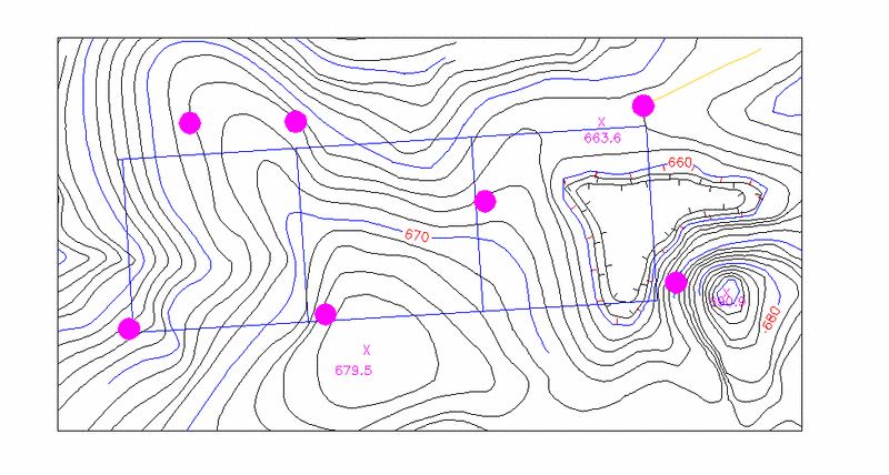
To verify contour elevations, and to check whether the top of the drillholes are close to the contour grades of the contours, use Drawing Inspector under the Inquiry pulldown menu. You will notice that all the holes top out at just about the right elevation you would expect based on the nearby contours, the only slight exception being the slightly lower drillhole shown below, where some of the surface could have been removed where the hole was drilled. It’s just a few feet low:
Note also that if you inspect the blue boundary lines, they, too have elevation. Those lines should be set to zero using the command, “3D Entity to 2D” under Edit. Otherwise, they will impact surface modeling. It’s a good idea to turn off the Drawing Inspector when you are not using it. Also, by right clicking with the mouse button when Drawing Inspector is on, you can change what you inspect (layers versus elevations, for example).
Step
2—
Set up
Strata Definitions to Colorize the Strata
This is a one-time process. The Strata Definitions file is used by
Draw Geologic Column and by Fence Diagram and by the routines that
color and display the block model. It can also impact tonnage
calculations, because you can set the strata density within Strata
Definitions. The dialog appears as shown below. The asterisk can be
used to apply the definition to anything that begins with the
letters preceding the asterisk. In this way, Standard Buff with
Vertical Seam would be treated as all the other Standard Buff
strata in terms of coloring and modeling.

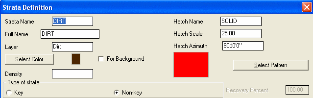
The columns to be shown in the spread sheet can be set using Column Options. The values can be edited with in the spread sheet shown above or by selecting the strata row and using Edit button. You see more settings that can be changed.
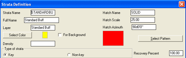
Contrast the StandardBuff settings with those for Dirt, which we have colored black and designated “Non-Key”, which means it is waste, not a product you are mining.
Step 3—Draw
Geologic Column
Once you have verified your colors for the strata (again, a
one-time process using Strata Definitions), it is valuable to
confirm the quality of the drillhole import by drawing the geologic
column. One method is to draw the columns next to the drillholes.
So choose Draw Geologic Column at the bottom of the Drillhole
pulldown menu. Possible settings for the dialog are shown
below:

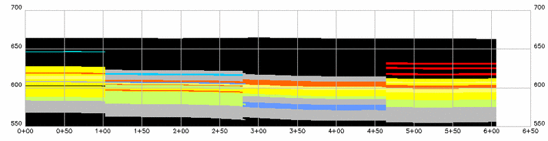
These settings produce the plot shown here:
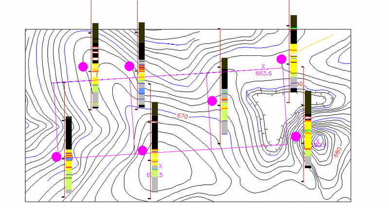
This is the first indication of the location of the yellow standard buff, as well as the location of silver grey and other colored zones. The location of the black overburden material is also clear in the plot.
Step 4—Assign a
Bed Name to All Strata
The block modeling routines
require that the various strata be organized into beds. You might
have a top 80-foot bed and a lower 100-foot bed in large deposits
of ore. If you don’t want to distinguish beds, just put all the
strata into one bed name, like Stone. Note that if a column “Bed
Name” was made in the original Excel file, all the strata could be
imported with a bed name and you’d be done. You might consider
removing the Ztop column in the original spreadsheet, and
substituting a Bed column with the name Stone in every entry, then
adjusting the custom import to bring it in. But to add Beds
“after-the-fact”, choose Assign Bed Names with Strata/Bed Utilities
under the Drillhole pulldown menu. Select all drillholes and enter
“Stone” for the bed name, for example. Enter N for No for “Use
Parameter Filter”. Then select all strata in the list at right.
Highlight and click OK. Done.

Step 5—Surface
Mine Reserves
You are now ready to get a volume of any material desired. Before
you do the command, you will need a closed polyline perimeter. Note
in the above graphic plot with contours, we have 3 blue squares,
that might be areas of interest for volumes. Each might represent a
mining block. But in reality, these are not closed polylines, but
are drawn as individual polylines in approximate N-S and E-W
directions. To create closed polylines where the zone of interest
is “enclosed” by other polylines, a useful command is “Boundary
Polyline” under Draw. Choose this command.
Pick all the blue polylines that “bound” the rectangle of interest (or that bound all the rectangles). Do not pick any contours or other polylines. Enter a snap tolerance of 1 (to “bridge” gaps of up to 1 foot). Enter the layer to draw the polylines in (CLAYER would put them in the current layer). Then pick inside, and the closed, rectangular polylines are drawn.
Now run the command Surface Mine Reserves under the Stratacalc pulldown menu. Fill out the dialog as shown, being sure to select “Block Model” method. This selection does an “on-the-fly” block model. The Geologic Model selection would work from a stored Geologic Model file, which can be a block model or a strata-based model. Specify the block by elevation, entering the bottom and top of the zone of interest (we did 580 to 620 here).

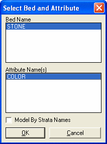
Also be sure to select “Calculate Strata Qualities” and “Breakout Quantities by Attributes”, options near the bottom left of the dialog. After you select all 7 drillholes to model (you can crossing select the entire screen, as only drillholes will be selected and the rest filtered out), you will get this dialog:
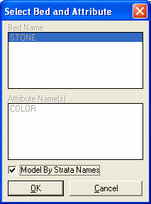
You can “Model by Strata Names” or by Color, since the Color attribute is the strata name! Next you can pick any of the strata to report, by selecting them:
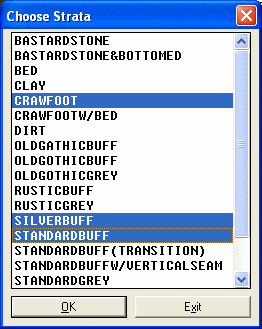
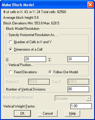
If we choose Crawfoot, SilverBuff and StandardBuff, quantities will be calculated for that block. Next you pick the limits of the study area, from lower left (well below and left of the drillholes) to upper right (well above and to the right of the drillholes) and set your gridding resolution. Figure if you have 40’ of elevation range, 80 vertical zones will give you about 0.5’ per zone for analysis.
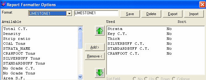
Pick one of the inclusion perimeters, and you are taken to the “Report Formatter” as shown below. Here it is shown as it might appear with a fresh installation of Carlson, completely unformatted.
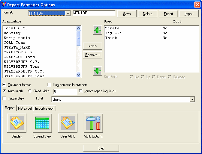
Move to the right the Silverbuff C.Y., the Standardbuff C.Y. and the Crawfoot C.Y. You can name the format in the upper middle box as Limestone1, so it is a report option available to you in the future (see below):
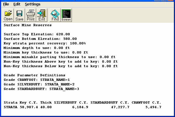
Click Display in the lower left of the screen, and you get the first report:
Step 6—Reporting
in Cubic Feet: Making User-Defined Attributes for
Reporting
When configured to “English” units, that is, feet, the program
defaults volumes in the form of cubic yards. If you wanted to
output cubic feet, then the default output variable for cubic yards
needs to be multiplied by 27 to produce cubic feet. The variables
“known” to the program can be listed, within the Report Formatter,
by clicking the Attribute Options button at the bottom of the
screen. A formula must be created for all of the named strata to
convert cubic yards to cubic feet. Therefore, to obtain all of the
strata in the Report Formatter, it is necessary to re-run Surface
Mine Reserves using the same settings in the dialog, but when
prompted for Choose Strata, select all of the strata, as shown.
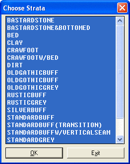
Then when you press OK and complete the gridding process, all of the strata appear in the Report Formatter, either in the left or right column.
The next step is to click the User Attribute button at the bottom of the screen, which then produces the following dialog:
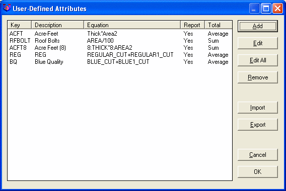
A few conversions are provided by default. We will need to add a conversion to Cubic Feet for each strata of interest. To begin, click Add.

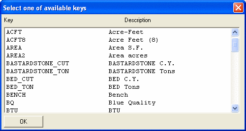
For the example of “BastardStone”, you simply multiply the “known” variable for BastardStone by 27 to calculate cubic feet. Whatever is filled out for Description is what appears in the report. To see what the program uses as “known” variables, you click “List keys”. The variable can be directly selected from this dialog, then the “*27” can be appended in the equation. Items are listed alphabetically:
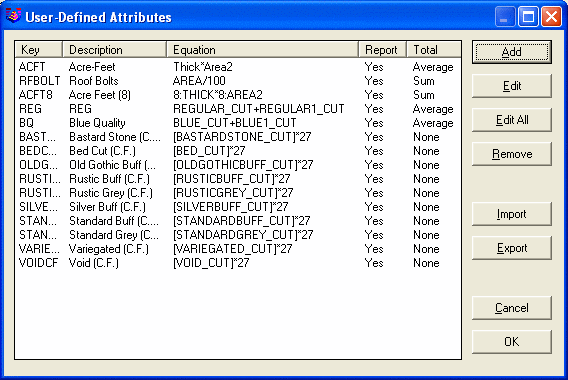
Repeat for each of the stone types involved. The pattern is, every time you click Add, click List Keys, choose the next stone of interest (e.g. BED_CUT), multiply by 27 in the equation, fill out the new “key word” for the cubic feet variable, fill out the full description for reporting and the decimal places, consider whether to Total by Sum, use No Total, etc., then click OK. Repeat for each strata. In order to see “Crawfoot” as a strata, you may need to select a larger number of vertical divisions, to “reveal” the very thin Crawfoot seam and get it in the list. Note that this is a one-time process. The new key variables will always be retained on future work. The final table might appear as shown below:
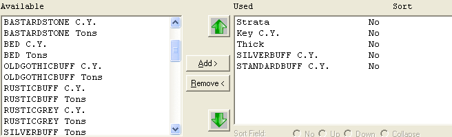
Next, click OK and return to the Report Formatter. More the generic “Strata” and cubic yard items from the right column back to the left column and move all the desired cubic feet elements over to the right-hand column and save this new format as Limestone2.
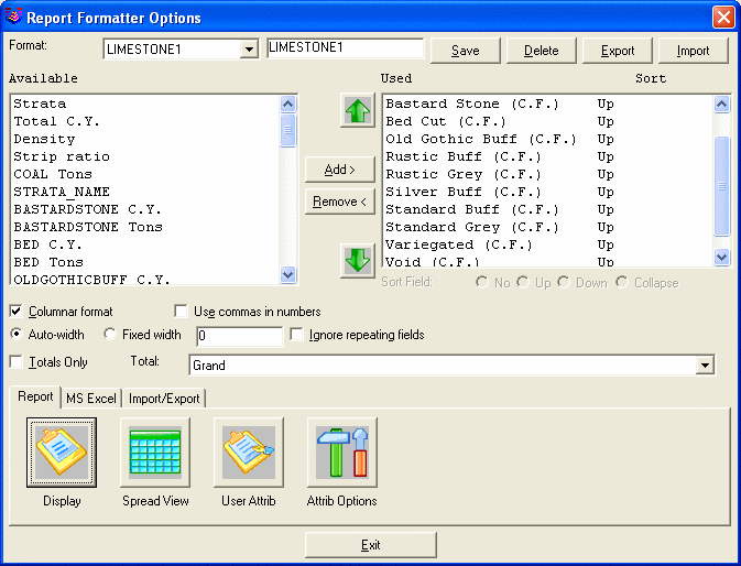
Note that using the “User Attrib” button, you can make new elements for reporting, and these elements, like Standard Buff (C.F.), can be used in equations themselves, using their “key word” designation (“STANDARDBUFFCF”). Thus the Report Formatter can be used to produce all sorts of outputs and reports, all deriving from the known elements in the original report. To see results directly in Excel, click the “MS Excel” tab then click Export to Excel at the lower right of the dialog:
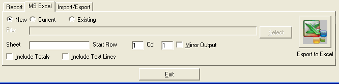
This leads to reporting directly in Excel:

Step 7—Viewing the
Ore Body Model in 3D
So far, we have produced volumes of material by “on-the-fly”
calculations. We have not created a block model of our strata. The
block model has only been created internally by the program based
on the selection set of drillholes. An official “block model” is
made by the command “Make Block Model” at the top of the Block
Model pulldown. Select that. Here again, you can make the block
model directly from the strata names.
Choose the lower left corner of the grid by the “Pick” method, and using the “end” snap (for endpoint) pick the lower left corner of the site, then the upper right corner of the site, as defined by the rectangular polyline enclosing all contours. Then set the grid resolution as shown below. Since we are dealing with “named” strata that abruptly transition to another form, use the “discrete” method of modeling. Note that for ore bodies, where qualities are typically modeled, “inverse distance” or “Kriging” are more typical modeling methods.
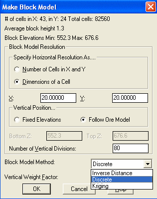
Note also in the dialog above that you can set the vertical position for modeling at fixed elevations or you can follow the ore model. The “follow” method finds the top and bottom of the ore material, then divides the vertical positions as defined, here by 80 divisions. So if the ore material narrowed, then 80 divisions would narrow to a smaller dimension. If you want fixed vertical dimensions, choose “Fixed Elevations”. After you click OK, select all strata to process, and name the block model to be created. Also create, for later use, the grade parameter file and Geologic Model grid model. Click “Yes” to both the options below:
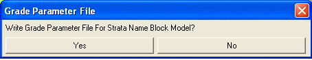
These options occur only when choosing the “Model by Strata Name” option above. Otherwise, you must use a pre-made Grade Parameter File and make the Geologic Model file by a separate process. The Grade Parameter File sets the colors (and even pricing) for the named strata or quality zones (in the case of attribute-defined grades). Making the Grade Parameter File this way does not set colors that match the colors set in Strata Definitions. You will need to run the command, “Define Grade Parameters” under the Ore pulldown menu and change the colors to match what were used in Strata Definitions, for consistent viewing, so that the 3D Views match the colors in Draw Geologic Column, for example.
Now run Block Model 3D Viewer under the Ore pulldown, choose the “blk” Block Model File and the “gpf” Grade Parameter File, press “OK” at the Block Model Viewer dialog, then select a perimeter for viewing. You obtain a plot as shown below:
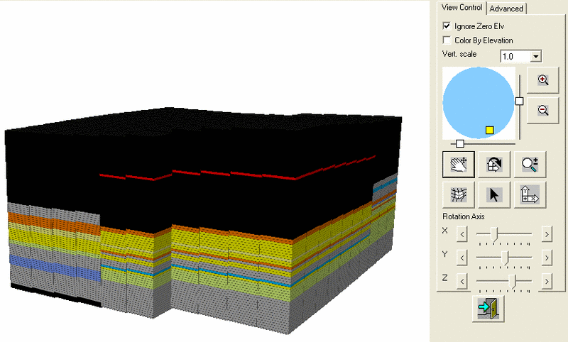
Note that you can exaggerate the vertical scale, or using the “Advanced” tab, you can switch from rendered view (above) to “Leave as Points” view. If you switch from Rendered to Points viewing, you must Exit the screen view (lower “exit door” icon) then repeat the command. Note that the yellow “Standard Buff” stone shows clearly in the 3D Block View, as does the red Void zone within the upper portion.
Step 8—Viewing the
Ore Body in Profile View (Fence Diagram)
The process of making the Block Model was critical not only for 3D
Viewing but also for the Profile View or “Fence Diagram”. The 3D
View used the “blk” file but the Fence Diagram command makes use of
the “Geologic Model” or “pre” file as well as the “blk” Block Model
File. Now that we have these, from Step 7 above, we can do the
Fence Diagram. Before issuing the Fence Diagram command, draw a
polyline through the drillholes or across the site that you will
pick for the profile view of the strata (stone). Select Fence
Diagram under the StrataCalc pulldown menu. Fill out the dialog as
shown below:

You could choose to exaggerate the vertical scale by changing the vertical entries to 20 rather than 50 (scale, grid interval and text interval). Then pick the polyline to use for the profile, and the “Geologic Model” and the ”grade parameter file” as prompted. A typical result is shown below: