Case Study: Block Modeling by Quality Attributes
This tutorial takes a set of drillholes and goes through the steps
that create the block model. The different grades are defined in
the Grade Parameter File. Blocks are drawn and viewed in 3D for
analysis. Cross sections are cut through the blocks and volumes by
grade are calculated with Surface Mine Reserves. Finally, the
Optimized Pit Design is found with the Lerch-Grossman
algorithm.
Drawing with Drillholes
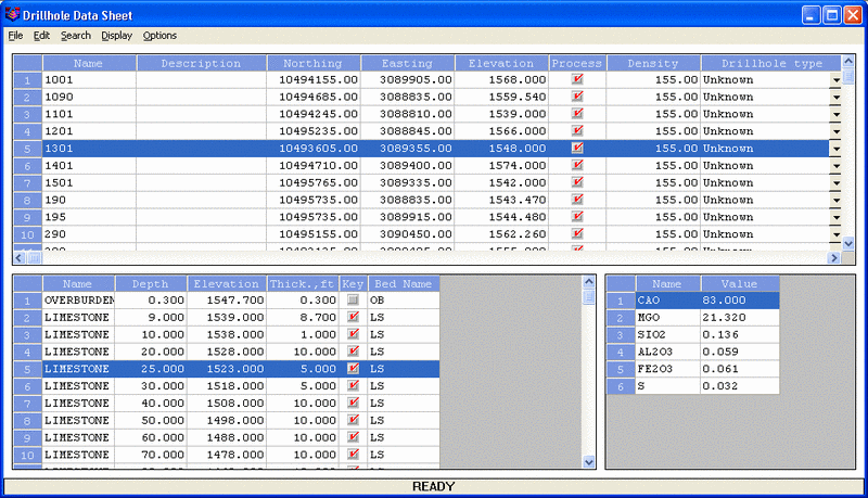
The first step is to import the drillholes and name the beds based
on how the seams are to be modeled. This example is a limestone bed
with a thin layer of overburden, so there are just two main
material types in the drilling, OB and LS are the bed names. The
drillholes have already been imported for this example. That
process is documented in other documents. There are 16 drillholes
in this drawing. The drawing name for this tutorial is Block Modeling.dwg. Shown here are the
plan view of the topography and the drillholes, and also the
drillhole datasheet to display the drilling data. 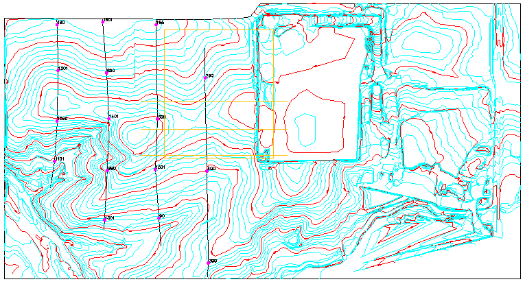
Make Block Model
This command is used to create the block model from the drillholes.
The first selection is to choose the Bed Name to model, and then
the quality or qualities. Just one quality attribute may be used,
or several at once. In this example, the LS bed and the CaO
attribute will be modeled, as shown in this window. It needs a grid
file to set the horizontal block sizes, so either pick the position
from screen, and put in a dimension for X,Y, or copy an existing
grid for positioning. For this one, the Surface Topo.grd can be copied for a
position, which is 20x20 in dimension. 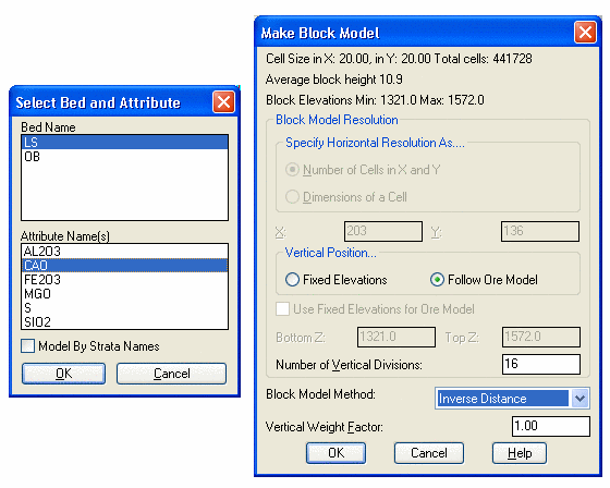 The second window sets the block height and
modeling method. There are two distinct methods for setting the
block height. They can be set to a fixed elevation and size which
is independent of the beds, or can follow the top and bottom of the
ore model from the drillholes. This creates almost a stratified
block model where the elevations of the blocks follow the top and
bottom of the ore elevations. This is like a hybrid of both
strata and block modeling. If there are not any strata, such as in
a gold or copper deposit, then the Fixed Elevations method is
preferred. Both methods work the same. If using the Fixed
Elevations method, to set the block height, the top and bottom of
the model are entered, with the number of samples chosen to set the
average block height, which is calculated and displayed at the top.
In this screen, if the Number of Vertical Divisions is set to 16,
the average block height listed above is 10.9. This should work
well with the horizontal size of 20x20, giving an average block
size of 20x20x10. This example will use Inverse Distance as the
modeling method with a vertical factor of 1. Selecting OK builds
all of the blocks and puts them in the BLK file. Choose a name for
the BLK file, such as LS_CaO.BLK.
The second window sets the block height and
modeling method. There are two distinct methods for setting the
block height. They can be set to a fixed elevation and size which
is independent of the beds, or can follow the top and bottom of the
ore model from the drillholes. This creates almost a stratified
block model where the elevations of the blocks follow the top and
bottom of the ore elevations. This is like a hybrid of both
strata and block modeling. If there are not any strata, such as in
a gold or copper deposit, then the Fixed Elevations method is
preferred. Both methods work the same. If using the Fixed
Elevations method, to set the block height, the top and bottom of
the model are entered, with the number of samples chosen to set the
average block height, which is calculated and displayed at the top.
In this screen, if the Number of Vertical Divisions is set to 16,
the average block height listed above is 10.9. This should work
well with the horizontal size of 20x20, giving an average block
size of 20x20x10. This example will use Inverse Distance as the
modeling method with a vertical factor of 1. Selecting OK builds
all of the blocks and puts them in the BLK file. Choose a name for
the BLK file, such as LS_CaO.BLK.
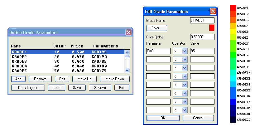
Define Grade Parameter File
This command defines the grade ranges of the ore. This is what
defines the blocks for colors and divisions for cross sections and
volumes. There is a Draw Legend button to put it on the map. The
price per pound is also defined here for the cost model, and that
will be used for the optimized pit design. Also notice that there
are 8 blanks for the various Parameters where the combination of
the several attribute ranges can define the grade. For example the
CaO > 90 and MgO< 15 defines the "High-Grade". For this
example, just the CaO is defined for the different ranges. If
another range is already defined, then the program will just use
what is available. That is why just the ">" option is used
below, starting at the highest grade and working down.
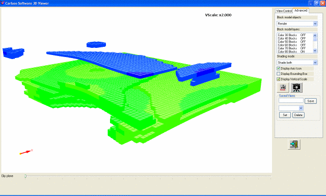
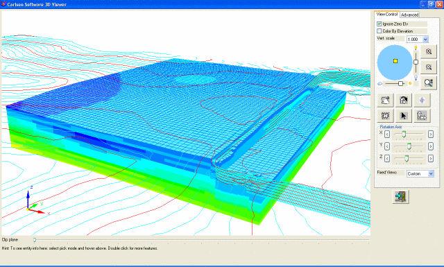
 Block Model Viewer
Now that the block model is built and the grade ranges are defined,
the model can be inspected and viewed in 3D to check it for any
problems. If the model is large, it is best to use an inclusion
polyline to view just a subset of the entire model. In the Advanced
Tab, there is a way to turn the various blocks on and off like
layers. Just click on the line to turn on or off and the blocks are
removed or added from the screen. This allows 3D views to see what
the quality is inside the middle of the blocks. Notice in this
example there are just green and blue blocks remaining. 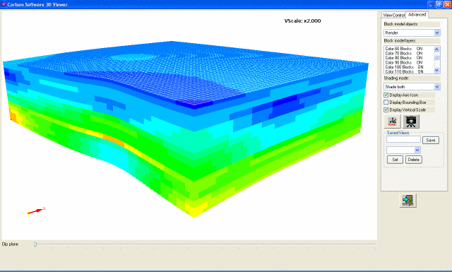
Draw Block Model
This is not a required step, but is convenient to place the blocks
in the drawing permanently. This command will draw the blocks on
screen in CAD as nodes or “dots”. These nodes can then be brought
into the 3D Viewer window and rendered the same as the Block Model
3D Viewer does. The nice option in this command allows to have a
top and bottom limiting surface to crop the blocks. That way if
just the blocks on a certain bench want to be viewed, use just the
top and bottom grids of that bench, or even the topography, and an
inclusion perimeter, to contain the blocks to draw, and ultimately
view. After selecting the file, just leave all set to "YES" on the
Draw Block Model screen. The nodes and contours drawn in CAD can be
viewed with the 3D Viewer Window as seen below. 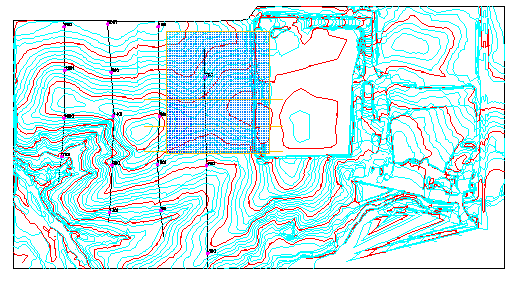
Define Geologic Model
This step is necessary to combine the block model with the surface
topo and any top or bottom elevation surfaces that will make up the
entire model. The procedure for strata models is to just add the
elevation grids as normal, and then add the BLK block model file to
the appropriate interval. Flat elevation grids can be used for
this, if it isn’t a stratified model that has roofs and floors,
like many hard rock metal mines and quarries that aren’t
stratified. 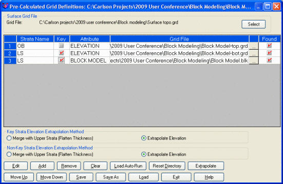
Fence Diagram
Now that the entire model is built and checked, a Fence Diagram can
be drawn to see the geology and blocks in section view. Fence
Diagram has an option to Hatch by Block Model. This can be drawn in
two ways. The initial section shows it on a 2D Grid, the second one
can be seen in 3D where it draws and hatches the fence in 3D below
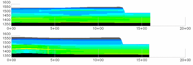
the line, in Real World Coordinates. Shown below are two fence
diagrams from the drawing, on a 2D grid. Notice the coloration of
the blocks based on grade of limestone. 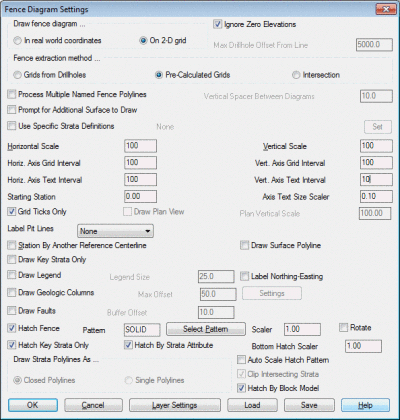
 There is also an option to draw the
Fence Diagrams in 3D using the Real World Coordinates setting. When
this is viewed in the 3D Viewer Window along with 3D Geologic
Columns, the result is very useful to visualize the geologic
deposit as shown below. The Draw Geologic Column command will draw
the drillholes as 3D columns, and they can also be colorized by the
Grade Parameter File. Notice how the coloration in the drillholes
corresponds to the coloration in the fence cross-sections,
indicating and good modeling estimation.
There is also an option to draw the
Fence Diagrams in 3D using the Real World Coordinates setting. When
this is viewed in the 3D Viewer Window along with 3D Geologic
Columns, the result is very useful to visualize the geologic
deposit as shown below. The Draw Geologic Column command will draw
the drillholes as 3D columns, and they can also be colorized by the
Grade Parameter File. Notice how the coloration in the drillholes
corresponds to the coloration in the fence cross-sections,
indicating and good modeling estimation. 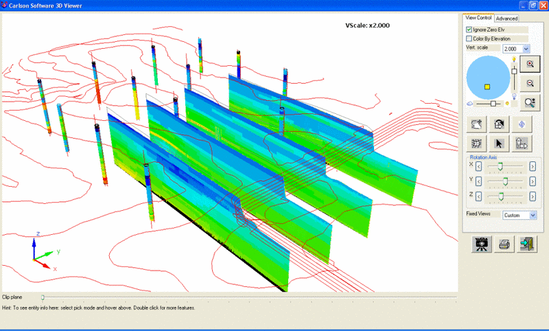
Surface Mine Reserves
The next step is to get the volume and tons of the different grades
of limestone with the Surface Mine Reserves. There is one check box
to turn on that will report the tons by grade, it is Breakout
Quantities by Attributes. This will not only give total tons of the
limestone, but also the tons in the various grades. Here is how the
window should appear. 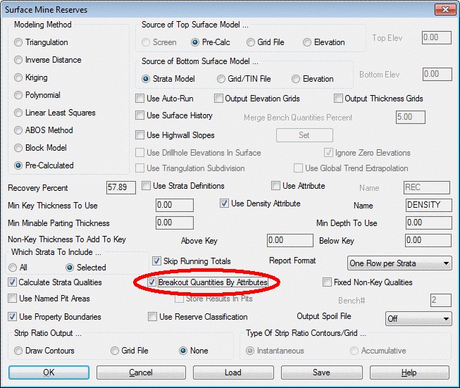 Shown here is the report of the data
dumped into Excel using the Report Formatter. Notice how the total
Key tons match the individual grade tons added up in the yellow
cells. This is a good check to make sure all grades are accounted
for in the report. Also confirm that each grade's CaO falls in line
with the values defined in the Grade Parameter File.
Shown here is the report of the data
dumped into Excel using the Report Formatter. Notice how the total
Key tons match the individual grade tons added up in the yellow
cells. This is a good check to make sure all grades are accounted
for in the report. Also confirm that each grade's CaO falls in line
with the values defined in the Grade Parameter File. 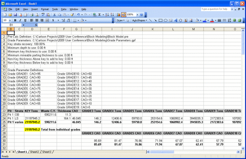
Prepare Value Block Model
Now to find the optimized final pit of profitable mining, we will
run this command to create a value block model, where each block is
assigned a cost associated with it. Once this value block model is
created, then the Optimized Pit Design can be run. First, select
the geologic block model to analyze. This is the file used in the
steps above. Then choose either to use the Grade Parameter file, or
to Enter the parameters on screen here. For this run, the Economic
Parameters will be entered. Select the Surface
Topography grid when prompted to do so. It will use this to
calculate the overburden on top of the blocks. 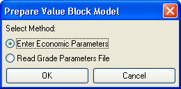 Enter in the Economic Parameters. Shown here is
a sample of the costs associated with the various mining stages.
This writes the value block model, where each block now has a value
assigned to it whether it is profitable or not. This file is named
Value Block Model.BLK.
Enter in the Economic Parameters. Shown here is
a sample of the costs associated with the various mining stages.
This writes the value block model, where each block now has a value
assigned to it whether it is profitable or not. This file is named
Value Block Model.BLK.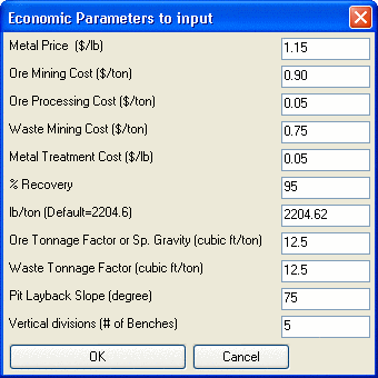
Optimized Pit Design
Now that the Value Block Model is written, the Optimized Pit Design
is run to create the ultimate pit and create the ultimate pit block
model. The Value Block Model is now the file to process, and this
one is selected first. All options are turned on to create an
ultimate pit grid, block model and a report. The block model is
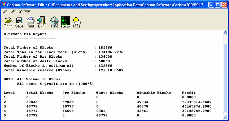
just for calculation purposes and contains cost values. 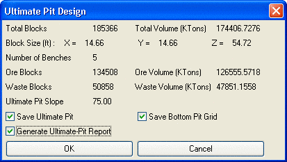 The final report shows that most of the blocks
are mineable. Level 1 doesn't have anything in it that is mineable.
The lowest level, 5 is not mineable, though there are blocks in it.
The blocks that are not profitable are what is left in the image
below. The grid is displayed here, with the Surface 3D Viewer, and
colored by elevation. It is easy to make changes in the input
parameters and run it again. The cost to mine or process the ore
can be modified and the new cost model created to see how it
affects the output.
The final report shows that most of the blocks
are mineable. Level 1 doesn't have anything in it that is mineable.
The lowest level, 5 is not mineable, though there are blocks in it.
The blocks that are not profitable are what is left in the image
below. The grid is displayed here, with the Surface 3D Viewer, and
colored by elevation. It is easy to make changes in the input
parameters and run it again. The cost to mine or process the ore
can be modified and the new cost model created to see how it
affects the output. 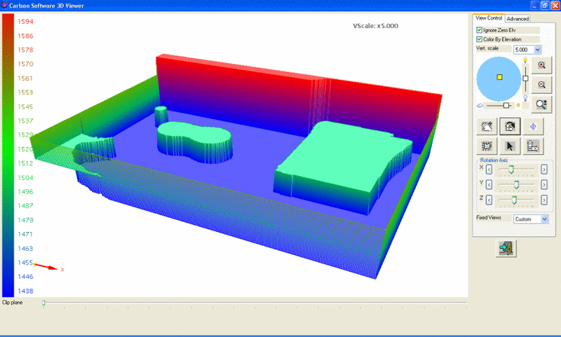
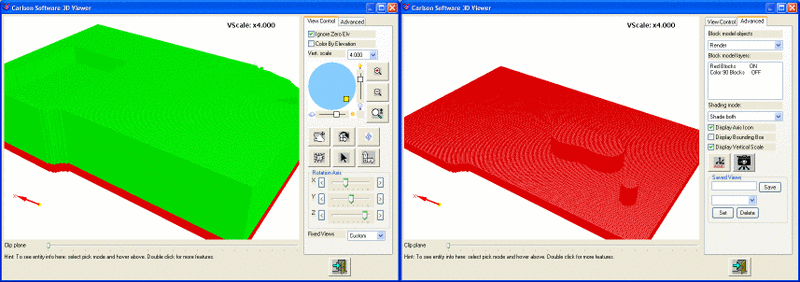
 There is an automatic Grade Parameter File
written called the Profit and Loss.GPF. This will colorize the
blocks in the Value Block Model green if they are profitable, and
red if they are not. This final model can also be viewed in 3D and
it will resemble the ultimate pit grid file. Shown below is the
full model, and then the profitable blocks are removed or "frozen"
and just the red, nonprofitable blocks remain.
There is an automatic Grade Parameter File
written called the Profit and Loss.GPF. This will colorize the
blocks in the Value Block Model green if they are profitable, and
red if they are not. This final model can also be viewed in 3D and
it will resemble the ultimate pit grid file. Shown below is the
full model, and then the profitable blocks are removed or "frozen"
and just the red, nonprofitable blocks remain.