Prepare Value Block Model

This command creates a block model that represents the economic value of each block. The value block model is made by loading in one or more .blk files and then applying user-defined equations to determine the value of each block. The value block model may then be used with the Optimized Pit Design command.

When the command is first executed, you will be prompted to select a .blk file. Then the below dialog will appear where you may add additional .blk files. The .blk files will be automatically sorted according to the average elevations of each file. These average elevations are calculated from the upper and lower elevation grids in each .blk file.

After clicking OK, the below dialog will appear.

Any attributes from the input .blk files will be listed on the left side of the dialog. These attributes may be used when writing equations to define the value of each block. Note that when these attributes are referenced, it refers to the value of each block individually - these are not average values for the block model as a whole. In addition to the attributes in the .blk files, two additional attributes will always be generated: Z_centroids and Volume.

The Z_centroid attribute is the elevation of each block's centroid.
The Volume attribute is the volume of each block, as measured in cubic feet/meters.

Calculate: This button will calculate the value block model according to an equation file (.db3 file). Note that this button does not save the results. You must use the Save Model button to save the results to a .bm file.

Define Equations: This button will allow you to create an equation file (.db3 file). Additional information about this function is provided below.

Set Attribute as Value: This button will set the currently selected attribute as the economic value for each block in the value block model. Note that this button does not save the results. You must use the Save Model button to save the results to a .bm file.

Export GsLib File: This button will export the value block model to a .txt file in a GsLib format.

Save Surface TIN: This button will create a .tin file of the surface of the value block model. Note that this surface will have a block-like appearance and will therefore differ from the original upper limit of the input .blk files.

Save Model: This button will save the currently calculated value block model to a .bm file. This .bm file may be used as the input for the Optimized Pit Design command.

Define Equations Dialog

After clicking the Define Equations button, the below dialog will appear. After saving this table to a .db3 file, you may return to the previous dialog to calculate the value block model.

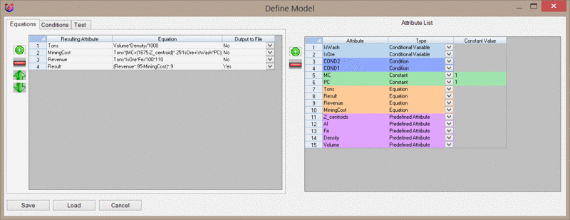
The dialog will first appear with only one Equation and Predefined attributes. All other equations, constants, conditions, etc. must be manually added.

Attribute List

The right side of the dialog lists all attributes. You can add or remove attributes with the two icons shown to the left of the list. Attributes may be one of five types, with each type showing with a unique color for visual organization.

1. Predefined attributes are attributes that have been found in the input .blk file(s).
2. Equations are attributes that will be calculated when the value block model is created.
3. Constants are attributes that have a non-changing value.
   
4. Conditions are logical tests that determine which variables to use. For example, you may define a condition that sets the processing cost for a block based on grade.
   
5. Conditional Variables are used as a result when Conditions are checked. For example, when setting the processing cost of a block based on grade, the processing cost is the Conditional Variable.
   

When adding an attribute, the below dialog will appear. Here you can give the attribute a name and set the attribute type. You may also set any other relevant options for the selected attribute type.

Attributes may be renamed by clicking inside the cell of interest and typing a new name. When the name of an attribute is modified, the change will be reflected in the Equations and Conditions tabs on the left side of the dialog. You may also change the condition type by selecting an option from the pulldown menu in the Type column.

Equations Tab

The Equations tab will display all defined equations in a spreadsheet view.

The Resulting Attribute column lists the attribute being calculated by the Equation column. For example, if you have a Resulting Attribute named "Tons", the result of the equation column will be assigned to this "Tons" attribute.

The Equation column is where you will write the equation for the attribute being calculated. For example, if you are calculating the "Tons" for each block, the equation could simply read "Volume*Density". This can be read as "Tons equals Volume multiplied by Density", where Volume and Density are other defined attributes. Equations will be calculated in from top to bottom by row, and therefore equations may reference the results from previously calculated equations. For example, the equation on the row 2 of the equation spreadsheet may reference the result from row 1, but it cannot reference the result from row 3.

The Output to File column controls if the attribute is output to the resulting .bm file. By default, attributes will not be saved to the .bm file. If the .bm file is to be used with the Optimized Pit Design command, only the economic value of each block should be output to the .bm file.

One equation, "Result", will always be defined and output to the .bm file. This equation should always define the value of each block and should always be output to the .bm file.

The below operations and the corresponding symbol are supported in the equation column:

1. Addition "+"
2. Subtraction "-"
3. Multiplication "*"
4. Division "/"
5. Grouping of terms "(" and ")"

Conditions Tab

The conditions tab will display all conditions in a spreadsheet view as shown below.

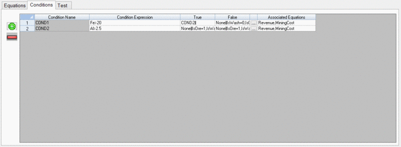
The Condition Name column lists the conditions in the order they were created. These cells are not editable.

The Condition Expression column is the logical test. In the above example, the first logical test checks if the block has an Iron content greater than 20%.

The True column lists the actions to take if the logical test is found to be true. At least two actions will be shown, separated by a vertical pipe. The first action tells the program which condition to evaluate next. The second action actually sets values to the Conditional Variables. In the above example, if a block is found to have an Iron content greater than 20%, the program will check Condition #2, but no Conditional Variable values will be assigned based on this test alone. If Condition #2 is found to be true, the program will not check another condition, but will assign the attributes "IsWash" and "IsOre" values of 1. This is similar to a nested "if" statement.

The False column lists the action to take if the condition is found to be false. This follows the same format as the True column. In the above example, if a block is found to have an iron content less than or equal to 20%, then no other condition is evaluated and the "IsWash" and "IsOre" conditional variables are assigned a value of 0.

If you click inside a cell of the True or False columns, the below dialog will appear.

This dialog sets values for the Conditional Variables based on the logic of the Condition. The two tables list Conditional Variables that will be affected by this Condition (IsWash and IsOre in this case). If the program needs to check another Condition rather than assign values to Conditional Variables as a result of this test, you may select the appropriate Condition to check below this Table. Conditional Variables may be added/removed from this list using the appropriate icons between the two tables.

The Associated Equations column lists the equations in which the conditions need to be evaluated. In the above example, both conditions will be evaluated when the Revenue and MiningCost equations are calculated.

Pull-down Menu Location: Geology Module > Block Model
Prerequisite: Must have an existing BLK file