Lesson 19: CADnet Paper Plan Digitizing to Volumes
This lesson transfers a paper plan into a DWG drawing using Carlson
CADnet and then uses Carlson Construction to calculate volumes from
the digitized linework.
Step 1 (Setup):
To digitize from a paper plan in CADnet, you need to install the
Wintab digitizer driver. See Digitizer Setup in the manual if you
have not installed or have problems with the Wintab driver. If
Wintab is installed, then make sure your drawing board is on and
take the paper plan provided with the manual and place it on your
drawing board.

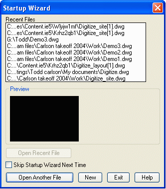
Click the icon for CADnet on your desktop or from the toolbar to
launch the program. You may be presented with a “Startup Wizard”
dialog similar to the one shown below, if so click New.
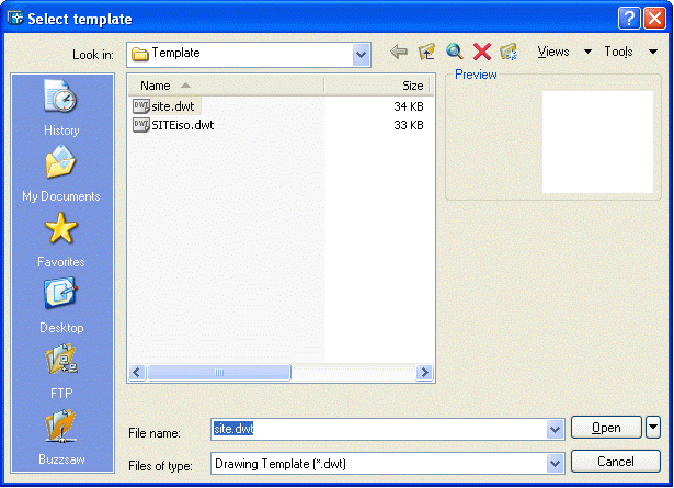
If a Startup Wizard did not appear, then under File menu, select
New to start a new drawing. You will be prompted for a template to
use. Templates determine the default settings for your drawing. For
this tutorial, select site.dwt or carlson.dwt and click Open.
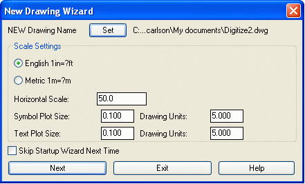
Next, the New Drawing Wizard appears for setting the drawing name.
Click on the Set button at the top dialog. In the file selection
dialog, enter the file name of "digitize" and pick the Save button.
Then Exit the New Drawing Wizard. From here, a Data Files
dialog appears where no changes are needed. Pick the Exit
button.
Step 2 (Tablet Calibration):
To start things off, you need to set the coordinate system for the
paper plan by running the Calibrate command under Digitize menu and
sub-menu Tablet. Calibration is required to let the program know
the orientation and scale of the paper plan.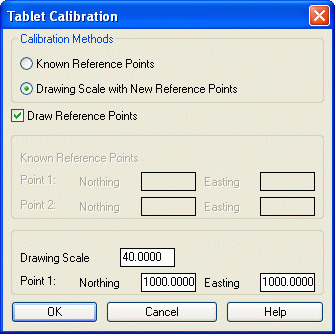
There are two different Calibration Methods: Known Reference Points
and Drawing Scale with New Reference Points. Known Reference Points
allows you to enter in the coordinates of two marked points on the
paper plan. This method applies when you know the coordinates of at
least two points on the paper plans. Drawing Scale with New
Reference Points allows you to setup a coordinate system for the
plans by entering the plan scale and picking any two points from
the paper plan with the digitizer puck.
In this case, we will use Drawing Scale with New Reference Points.
First, enter in the Drawing Scale listed on the paper plan. On this
drawing, the scale is 1:40, so enter in 40. Use the default
coordinates for Point 1 and click OK. Now Carlson Takeoff will
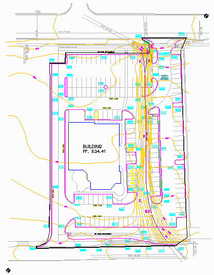
prompt you for your First and Second Reference points. Generally,
you want to pick to points on the drawing that you can find and use
again in case you need to recalibrate. Also, the further away the
points are from each other, the more accurate the coordinate system
will be. With the digitizer puck, pick on the  icon in the lower
left and upper right of the drawing for the two Reference Points.
The first point is assigned the coordinates of 1000,1000 from the
dialog and the second point is assigned coordinates to match with
the plan scale. From now on, all of your points will be in relation
to these two points.
icon in the lower
left and upper right of the drawing for the two Reference Points.
The first point is assigned the coordinates of 1000,1000 from the
dialog and the second point is assigned coordinates to match with
the plan scale. From now on, all of your points will be in relation
to these two points.
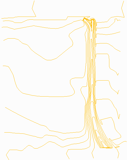
Step 3 (Digitizing Existing Contours):
We will now digitize the existing contours. The digitize routines
in CADnet can be used to populate the Existing, Design, and Other
targets used in Carlson Construction and the SiteNET portion of
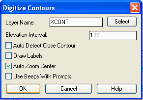
Carlson Civil. Under the Digitize menu, click on Existing. Next, go
to Digitize>Contour Polyline, and this dialog will appear. Enter
in a Layer Name of XCONT and select OK. Note: your Elevation
Interval should match the intervals marked on your paper drawing.
In this drawing, the interval is the same as the default of
1.00.
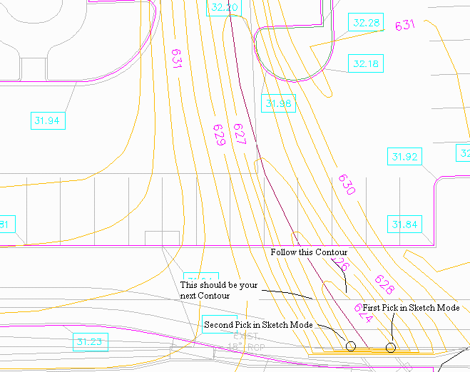
The rest of the prompting occurs at the command line and starts
with the contour elevation. Find the lowest elevation for the
existing contours labeled in bottom right corner of the paper plan
zoomed in on below. In this example, the lowest elevation is 624
feet. The elevation can be entered either with the digitizer puck
keys or with the computer keyboard. The layout of the digitizer
keys is set in Digitizing Settings->Puck Layout. Press Enter
after you have entered in 624. You want to enter in the lowest
contour so that as Carlson CADnet adds the Elevation Interval, it
is from lowest to highest.
Next, you will see the following prompt:
Sketch[0]/Exit[A]/Pick the first point:
There are two different ways to digitize: in Pick Mode or Sketch
Mode. You can switch between them at anytime. In this tutorial we
will run through how to do both. For now, type in [0] and press
enter to get into Sketch Mode. In Sketch Mode, you will be prompted
to Pick and drag. The point you pick is the starting point of a
contour. Drag is asking you to follow that contour with the
digitizer puck on the paper plan. Click a second time when you have
traced the entire contour and have reached the end of the contour.
You will then be prompted as follows:
Pick[0]/Close[A]/Undo[B]/Pick and
drag (Enter to end):
Type in [B] for Undo if you made a mistake and need to sketch part
of the contour again. [A] will close the contour, and [0] will
switch you into Pick Mode. We still have more existing contours to
digitize, so press Enter to end and answer yes to the Digitize
Another Contour prompt. Takeoff will prompt you to verify the
elevation. Remember, we set the Elevation Interval to one, so the
default elevation for your next contour line is 625, press Enter.
Now, pick the endpoint of the next contour and trace it in the same
manner as the previous contour.
Now let's try Pick Mode. Say yes to digitize another contour and
check to see if the default elevation corresponds with the contour
your about to digitize. If not, simply type in the correct number
in the command line. Next, pick [0] to get into Pick Mode. In Pick
Mode, you do not have to trace the contour. Rather, pick with the
digitizer puck to create points that will make up the contour.
Note: Less picks are needed on fairly straight segments.
Conversely, more picks will give you a more accurate contour. Press
Enter when you have reach the end of the contour. Repeat this until
you have digitized all of the desired existing contours (see
below).
Step 4 (Digitizing the Design):
Now we will digitize the building and curb linework of the Design
Surface using the Digitize 2D Polyline and 3D Polyline commands.
Besides drawing the linework positions, we will also assign layer
names to the linework that we will use later to identify the types
of linework. In this example, there are no design contours,
only the design building and curb linework and spot elevations.
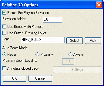
Let's begin by digitizing the main building. Under Digitize, check
on Design and go to 2D Polyline. 2D Polyline is used to digitize
linework entities with one elevation. Toggle off the check box
Use current drawing layer
and name the layer NEW BUILD. Toggle on the Prompt For Polyline Elevation option.
Then click OK.
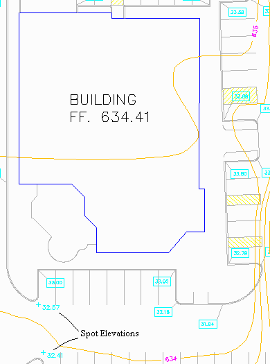
At the command line, enter in the building elevation of 634.41
found labeled in the middle of the building and press Enter. Then
pick the points that define the building outline. Start in the
upper left corner and pick at every corner around the building.
When you have picked around the entire building, type in [A] for
close to finish digitizing the building.
Enter polyline elevation
<0.00>: 634.41
First point:
pick a building point
Close[A]/Undo[B]/Osnap[.]/Pick
next point (Enter to end): pick >>>>>>> 1.8 the
next building point
Close[A]/Undo[B]/Osnap[.]/Pick
next point (Enter to end): pick the next building point
Close[A]/Undo[B]/Osnap[.]/Pick
next point (Enter to end): pick the <<<<<<<
Lesson_13_Digitizing.html last building point
Close[A]/Undo[B]/Osnap[.]/Pick
next point (Enter to end): A to close
Digitize Another NEW_BUILD
Polyline [Yes(A)/<No(B)>]? B for No
Notice that the parking lot linework consists of different
elevation levels. To digitize entities with more than one
elevation, go to Digitize and select 3D Polyline from the pull-down
menu. Make sure that the Prompt
For Polyline Elevation option is on, the Use current drawing layer toggle is off
and name the layer NEW EDGE ASPH.
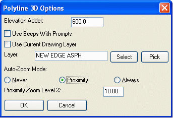
Let's start by digitizing the parking lot starting from the zoomed
in section below. The edge of asphalt is the inside line. The
parking lot elevation labels have been shortened on the paper plan.
For example, they read 35.37 and 35.12, when the actual elevations
are 635.37 and 635.12. Enter in 600 as the Elevation Adder, then
click OK.
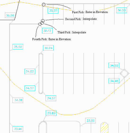
Click on the point with the digitizer puck where the 35.37
elevation label points to in the upper left corner of the parking
lot. When prompted for Elevation enter in 35.37. Pick below the
first point where the linework starts to curve. We do not have an
elevation for this point, but we can interpolate the elevation from
the two points around it using the interpolate option. Type in I
for interpolate or hit the A button on the Puck. Next pick the
middle point of the curve and again use Interpolate for the
elevation. Next pick the end of the curve at the 35.12 label and
enter in the elevation 35.12. Continue digitizing for the rest of
the edge of asphalt linework. Digitize each point where there is an
elevation label and each point where the curb line changes
direction.
The first prompts should resemble these:
First point: pick first point (at 35.37 label)
Interpolate[A]/screen
Pick/<Elevation[B]> <0.00>: 35.37
Z: 635.37
Close[A]/Undo[B]/Osnap[.]/Pick next point (Enter to end):
pick next point (start of
curve)
Slope/Ratio/Interpolate[A]/Degree/screen
Pick/<Elevation[B]> <635.37>: Press the
[A] button on the Puck for Interpolate
Slope/Ratio/Elevation[B]/Degree/screen Pick/Osnap[.]/Next point or
elevation<Interpolate>: pick next point (middle of curve)
This point elevation will be
interpolated upon completion.
Slope/Ratio/Elevation[B]/Degree/screen Pick/Osnap[.]/Next point or
elevation<Interpolate>: pick next point (end of curve, at 35.12
label)
This point elevation will be
interpolated upon completion.
Slope/Ratio/Elevation[B]/Degree/screen Pick/Osnap[.]/Next point
or
elevation<Interpolate>: 35.12 (Enter)
To check the elevations of the interpolated points go to Drawing
Inspector under the Inquiry menu and hover over the polyline you
just created. A window will appear showing you the layer name and
elevations along the line. If no elevations appear, right click and
check on Display Elevations.
Use the 3D Polyline command to digitize the rest of the parking lot
as seen below.
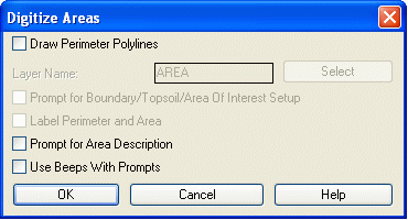
Step 5 (Area):
Now that we have digitized the Design Surface, let's check the Area
of certain sections. Select Area under the Digitize Menu and match
the below dialog.
To approximate the area of the main building, pick the points of
the building outline.
Command: dig_area
Pick starting point:
Pick points as close to the
building design linework as you can
Undo[B]/Pick next point (Enter to
end):
Undo[B]/Pick next point (Enter to
end):
Undo[B]/Pick next point (Enter to
end):
Undo[B]/Pick next point (Enter to
end):
Undo[B]/Pick next point (Enter to
end):
Undo[B]/Pick next point (Enter to
end):
Undo[B]/Pick next point (Enter to
end):
Undo[B]/Pick next point (Enter to
end):
Undo[B]/Pick next point (Enter to
end):
Undo[B]/Pick next point (Enter to
end):
Digitize Another Area
[<Yes(A)>/No(B)]? B
When finished with the building points, press Enter to end. Then
answer no for no more areas. Takeoff will then display an Area
report similar to the one shown below.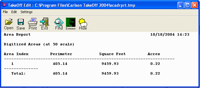
Step 6 (Spot Elevations):
In our paper drawing, we have two spot elevations labeled 32.57 and
32.41 shown in the bottom left below.
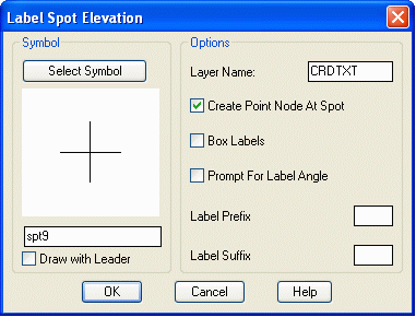
To digitize these elevations, we can use the Spot Elevation command
under the Digitize menu. Fill out the Spot Elevation dialog as
shown and pick OK.
In the paper plan, find and click on the spot elevations with the
puck. When prompted, enter in their corresponding elevations of
632.57 and 632.41.
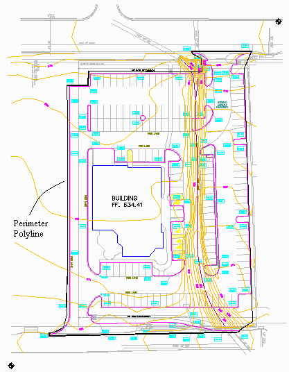
Step 7 (Boundary Polyline):
The limits of the site are defined by a closed polyline. This
polyline is used as the boundary for the models and the volumes.
Under the digitize menu, check on Other and then select Perimeter.
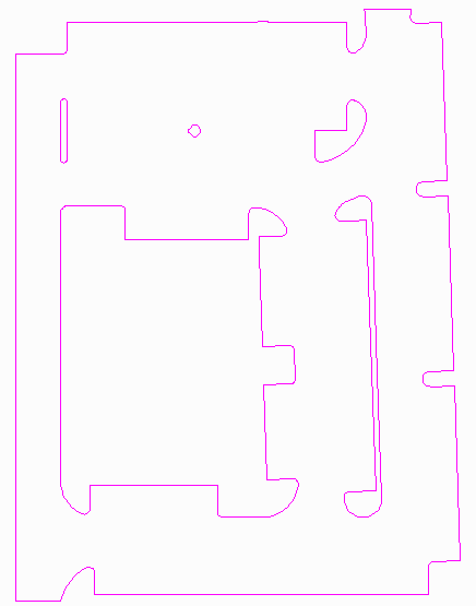
Type in PERIMETER as the layer name. Now digitize around the bold,
outside line shown below.
Say No to the prompt: Digitize
Another PERIMETER Polyline [Yes(A)/<No(B)>]?
Step 8 (Switch to Carlson Construction or Carlson Civil):
Now that we have digitized linework with CADnet, we can use Carlson
Construction or Carlson Civil to calculate Cut/Fill volumes and
material quantities. Run Takeoff->Boundary Polyline->Set
Boundary Polyline (command found under SiteNET in Civil) and pick
the perimeter polyline drawn in Step 7. This selected polyline is
now set as the boundary polyline for the rest of the Takeoff
routines.
Step 9 (Layer Targets):
From the Takeoff or SiteNET menu, choose
Define Layer Target/Material/Subgrade. Every entity (line,
polyline, point, etc) in the drawing is assigned a layer name.
Takeoff uses the entity layer names to define which entities are
for the existing ground surface, the design surface or no surface.
These surfaces are referred to as the “Target” surfaces. The
drawing entities are assigned their target surface by their layer
name. For example, if polylines representing design contours are on
the layer “NEW”, then “NEW” will be set as a layer for the design
surface. For layers of entities that are for neither existing nor
design surfaces (such as text labels for street names), the layer
target is set to Other.
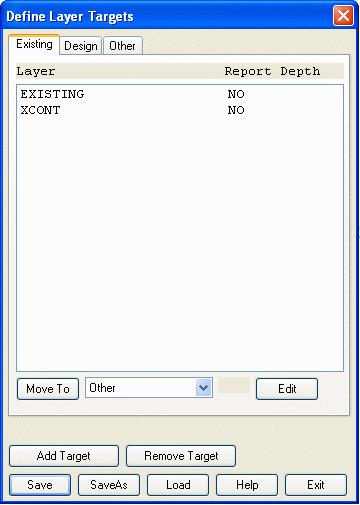
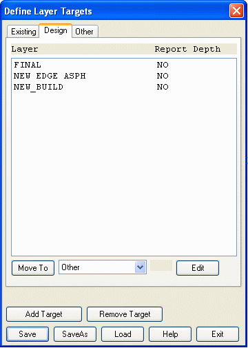
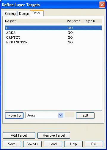
The Define Layer Targets dialog has three lists of layers:
Existing, Design and Other. To switch between lists, pick the tabs
at the top of the dialog. We have already defined the layers for
their correct targets. We did this by check on Existing, Design, or
Other in the pull-down menu.
Check that your Layer Targets resemble the
three lists shown here. If a layer is out of place, highlight it,
and hit the "Move To" button after selecting the correct target to
send it to. After reviewing, pick Save and Exit.
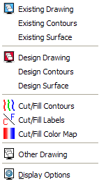
Now that the layer targets are defined, there
are several commands that can be applied. In the Display menu
(SiteNET in Civil), you can turn on/off whether to display layer
targets by using Existing Drawing, Design Drawing and Other
Drawing, or by right-clicking with your mouse.
Practice turning on/off the Existing, Design
and Other Drawing in the Display menu. When only Existing Drawing
is on, you should see just the contours. When only Design Drawing
is on, you should see just the design polylines and leader labels.
When only Other Drawing is on, you should see the entities that are
assigned to neither existing nor design.
Step 9 (Define Material/SubGrade):
Besides assigning target surfaces by layer,
layers are also used to define material names and subgrade depths.
By assigning material names and depths to layers, the volume, area,
length and count for entities on these layers can be reported. Also
the depth is used to vertically adjust the design surface. The
polylines used for subgrade depth must be closed polylines. Takeoff
supports nested subgrade polylines for exclusion areas such as
islands by counting how many subgrade polylines surround an area.
If the number is odd, then the area is inside the subgrade.
Otherwise the area is not part of the subgrade.
First, let's confirm the layer names for our subgrades. Go to the
Display menu and check on Design Drawing, uncheck Existing Drawing
and uncheck Other Drawing. Then run Inquiry->Layer ID and pick
the large pad polyline. It reports that this layer is NEW BUILD.
Next use Layer ID to pick the curb polyline. It reports that this
layer is NEW EDGE ASPH.
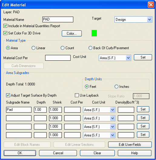
Now run Define Layer Target/Material/Subgrade
and pick the Design tab. Highlight layer NEW BUILD and pick the
Edit button. A dialog appears for defining the pad material
properties. Check on the Include In Material Report option, enter
the Material Name as “Pad”, set the first subgrade name to "Pad",
and set the Depth as 1. Once the dialog is filled out as shown,
pick OK.
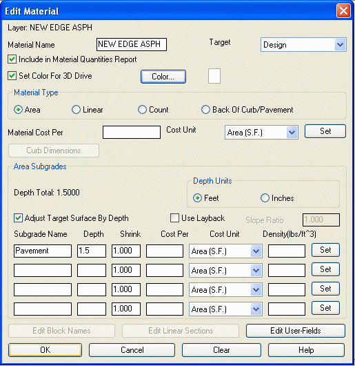
Next pick layer NEW EDGE ASPH and choose Edit. In the Edit
Materials dialog, check on Include In Material Report, set the
Material Name to “Pavement”, set the first subgrade name to
"Pavement", and set the Depth to 1.5. Then pick OK.
To save the subgrade changes, pick the Save
button on the Define Layer Targets dialog. Then choose Exit.
Now let’s visually verify the subgrade areas.
In the Takeoff or SiteNET menu, run Subgrade Areas->Hatch
Subgrade Areas. There is a dialog to select which subgrade to
hatch. Choose the Pavement. Then there is a dialog for the hatch
pattern and color. Change the color to green and click OK. Then run
Hatch Subgrade Areas again. This time choose Pad and set the hatch
pattern to Hex with blue color. The resulting hatch areas show
where the subgrade is applied. Notice how the islands are not
hatched because they are curb polylines that are already inside
another curb polyline. When finished viewing the subgrade areas,
run Takeoff->Subgrade Areas->Erase Subgrade Hatches.
Step 10 (Model Existing and Design Surfaces):
To calculate volumes, Takeoff needs two surfaces: existing ground
and design. These surfaces are modeled by triangulation. With
the preparation of the previous steps, we’re now ready to make the
models. To make the existing ground surface, run Takeoff->Make
Existing Ground Surface. The program will process the entities and
make the triangulation surface. Then to make the design surface,
run Takeoff->Make Design Surface.
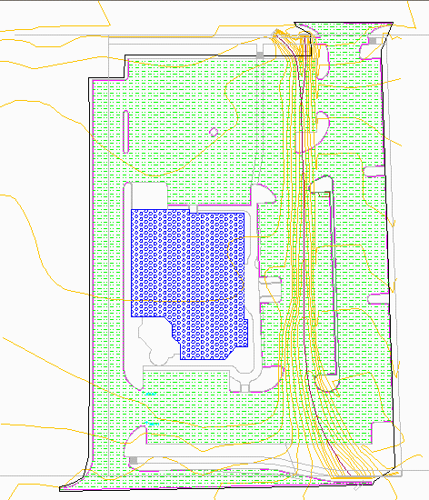
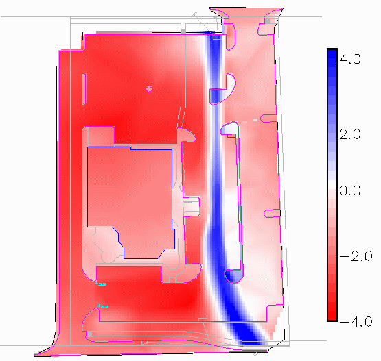
Step 11 (Cut/Fill Color Map):
Cut/Fill color maps can be used for a visual
output of the site cut/fill areas and also serves as a check that
the models are correct. In the Display menu, choose Cut/Fill
Color Map. Cut areas are drawn in different shades of red for
different depths of cut while fill areas are drawn in blue. To
change the resolution of the color blocks, run Display->Display
Options and change the Cut/Fill Color Map Subdivisions. This
parameter is the number of rows and columns of color blocks to
create. You can also draw a legend for the Color Map by going to
Draw, Cut/Fill Map Legend. Pick a point on your drawing to locate
the legend and press Enter. To turn off the color map, go to the
Display menu and pick Cut/Fill Color Map to uncheck it.
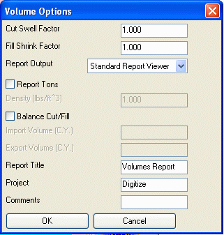
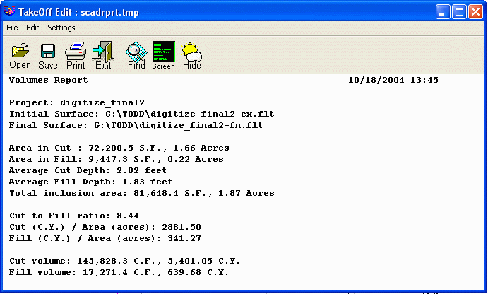
Step 12 (Calculate Volumes):
To calculate volumes, run the
Takeoff->Calculate Total Volumes command. There is an options
dialog for setting the cut swell factor and fill shrink factor.
These values get multiplied into the cut/fill volumes. Set these
factors as desired and click OK. Then the routine calculates the
volumes and display the report which includes the cut/fill volumes
and areas. The report can be printed or saved to a file. Pick the
Exit button to exit the report viewer.
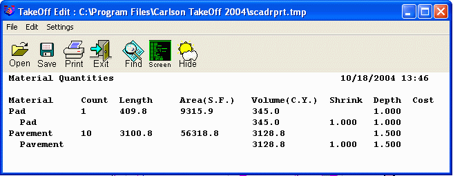
Step 13 (Material Quantities):
To report the material quantities, run the
Takeoff->Material Quantities->Standard Report routine. The
report includes the count, length, area and volume for each type of
material that was assigned for reporting in the Define Layer
Target/Material/Subgrade command. The Material
Quantities->Custom Report routine can be used to reporting these
values with control of the report format and the option to export
to Excel.