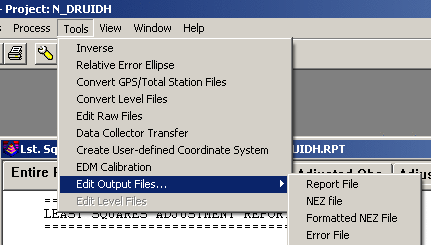
Inverse Buttons - The
'Inverse' button is found on the main window (the button with the
icon that shows a line with points at each end). You can also
select the Tools->Inverse menu option. This feature is only
active after a network has been processed successfully. This option
can be used to obtain the bearing and distance between any two
points in the network. Additionally the standard deviation of the
bearing and distance between the two points is displayed.
The Relative Error Ellipse Inverse button is found on the
main window (the button with the icon that shows a line with an
ellipse in the middle). You can also select the Tools >
Relative Error Ellipse menu option. This feature is only
active after a network has been processed successfully. This option
can be used to obtain the relative error ellipse between two
points. It shows the semi-major and semi-minor axis and the azimuth
of the error ellipse, computed to a user-define confidence
interval. This information can also be used to determine the
relative precision between any two points in the network. It is the
relative error ellipse calculation that is the basis for the ALTA
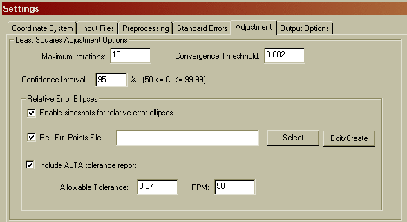
tolerance reporting. If the 'Enable sideshots for relative
error ellipses' toggle is checked then all points in the project
can be used to compute relative error ellipses. The trade-off is
that with large projects processing time will be increased.
If you need to certify as to the "Positional Tolerances" of your monuments, as per the ALTA Standards, use the Relative Error Ellipse inverse routine to determine these values, or use the specific ALTA tolerance reporting function as explained later in the manual.
For example, if you must certify that
all monuments have a positional tolerance of no more than 0.07 feet
with 50 PPM at a 95 percent confidence interval. First set the
confidence interval to 95 percent in the Settings/Adjustment
screen. Then process the raw data. Then you may inverse between
points in as many combinations as you deem necessary and make note
of the semi-major axis error values. If none of them are larger
than 0.07 feet + (50PPM*distance), you have met the standards. It
is however more convenient to create a Relative Error
Points File containing the points you wish to check and include the
ALTA tolerance report. This report takes into account the PPM and
directly tells you if the positional tolerance between the
selected points meets the ALTA standards.
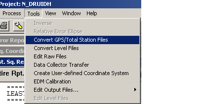
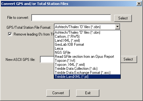
First choose the file format of the GPS vector file to be converted. Next use the 'Select' button to navigate to the vector file to be converted. If you are converting a Thales file you have the option to remove the leading 0's from Thales point numbers. Next, use the second 'Select' button to select the name of the new ASCII GPS vector file to be created. Choose the 'Convert' button to initiate the file conversion. Press the 'Cancel' button when you have completed the conversions. The file created will have an extension of .GPS. Following are the different GPS formats that can be converted to ASCII.
Ashtech/Thales: The
Ashtech/Thales GPS vector file is a binary file and is sometimes
referred to as an 'O' file. Notice that you have the option to
remove the leading 0's from Thales point numbers, by checking the
"Remove leading 0's from Thales point numbers" check box.
Carlson RW5: Carlson SurvCE version 2.0
or higher can store GPS vectors in the RW5 raw data file. Unlike
other vector files, these vectors are Antenna to Antenna so the rod
height information must be obtained from the RW5 file. This allows
you to edit rod heights and re-process the vectors. Additionally,
RW5 vectors are always in meters, regardless of the job units.
LandXML (.XML): The landXML
format is an industry standard format. Currently SurvNet will only
import LandXML survey point records. The conversion does not
currently import LandXML vectors.
GeoLab IOB Format: GeoLab's
vector format.
Leica: The Leica vector file is an ASCII format typically created with the Leica SKI software. This format is created by Leica when baseline vectors are required for input into 3rd party adjustment software such as SurvNet. The SKI ASCII Baseline Vector format is an extension of the SKI ASCII Point Coordinate format.
NGS G-File: The NGS G-File is
the format used National Geodetic Survey in their processing
software.
NGS G-File from an OPUS
report: Every OPUS report contains a G-File section. The
vectors making up this G-file are the vectors from the control
points to the computed. point making up the OPUS solution. These
OPUS vectors can be extracted and then combined with other GPS or
total station data to create a larger SurvNet project. If the OPUS
vector data is used in a SurvNet project it is important to use
Geoid modeling since the control points making up the OPUS solution
typically cover a large extents.
Topcon (.TVF): The Topcon Vector File is in ASCII format and typically has an extension of .TVF
Topcon (.XML): The Topcon XML
file is an ASCII file. It contains the GPS vectors in an XML
format. This format is not equivalent to LandXML format.
Trimble Data Collection (.dc): The Trimble .dc format is an ASCII file. It is typically output by Trimble's data collector. It contains a variety of measurements including GPS vectors. This option only converts GPS vectors found in the .DC file.
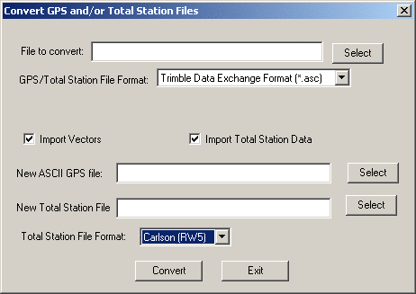
Trimble Data Exchange Format
(.ASC): The Trimble TDEF format is an ASCII file. It is
typically output by Trimble's office software as a means to output
GPS vectors for use by 3rd party software. The Trimble Data
Exchange file can also contain traverse data. The conversion dialog
will give you the option to create either an RW5 or CGR file with
the traverse data, along with the GPS file containing the vector
data.
Trimble LandXML (*.jxl): Trimble vector
files in Land XML format.
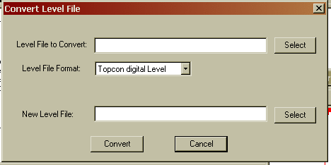
The purpose of this option is to convert differential level files from digital levels into C&G/Carlson differential level file format. At present the only level file format that can be converted are the level files downloaded from the Topcon digital levels.
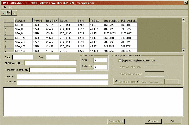
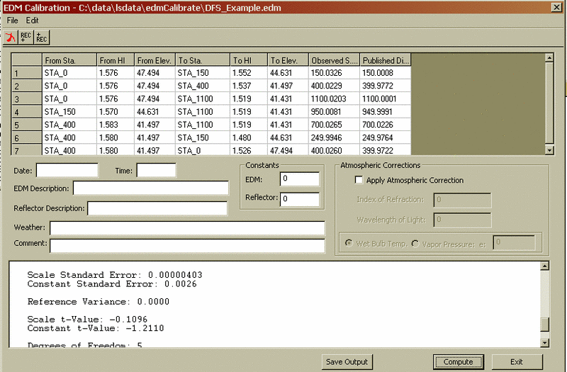
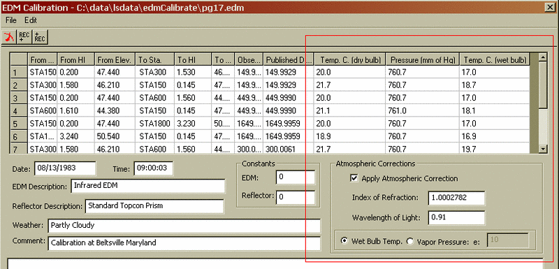
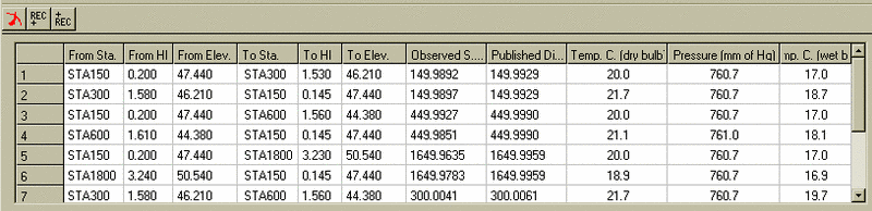
EDM Calibration Report
Observed Data
EDM Type:
Date: Time:
Prism description:
Weather description:
Comment:
Atmosphere Correction: OFF
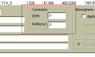
Constants: Refrector: 0.000 EDM: 0.000
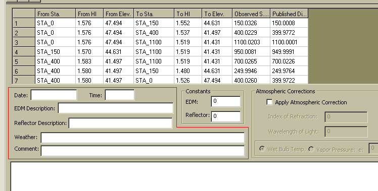
From From From To . To To Observed Published
Sta. Elev. HI Sta. Elev. HI Temp. Pressure Slope Dist. Dist.
STA_0 47.494 1.576 STA_150 44.631 1.552 0.0 0.0 150.0326 150.0008
STA_0 47.494 1.576 STA_400 41.497 1.537 0.0 0.0 400.0229 399.9772
STA_0 47.494 1.576 STA_1100 41.431 1.519 0.0 0.0 1100.0203 1100.0001
STA_150 44.631 1.570 STA_1100 41.431 1.519 0.0 0.0 950.0081 949.9991
STA_400 41.497 1.583 STA_1100 41.431 1.519 0.0 0.0 700.0265 700.0226
STA_400 41.497 1.580 STA_150 44.631 1.480 0.0 0.0 249.9946 249.9764
STA_400 41.497 1.580 STA_0 47.494 1.526 0.0 0.0 400.0260 399.9722
The above section shows the input. The input consists of the observed slope distances and the measured HI's. The from and To elevations are published data from the data sheet from NGS on the particular baseline being observed. The published distances are also published data from the data sheet from NGS. In this example atmospheric pressure was turned off so the temperature and Pressure fields are irrelevant.
ResultsNull Hypothesis, HO: EDM scale error and EDM constant error = 0.0
If the scale error and the EDM constant are 0.0 then the edm is without error. So the purpose of the statistical test is to test how close to 0.0 are the results.
Scale Error (ppm): -0.00000044
Constant Error: -0.0032
The two above lines show the values for the computed scale error and constant error.
Scale Standard Error: 0.00000403
Constant Standard Error: 0.0026
The two above lines show the values for the computed standard errors of the scale error and constant error.
Reference Variance: 0.0000126
Scale t-Value: -0.1096
Constant t-Value: -1.2110
Degrees of Freedom: 5
Critical t-Value at the 1 percent confidence level: 4.0320
Cannot reject the H0 for the scale error. (The scale factor is 0.0)
Cannot reject the H0 for the constant error. (The constant is 0.0)
The above lines show the final results of the statistical test. Since the test determined that we cannot reject the null hypothesis, this edm is in good working order.