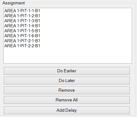
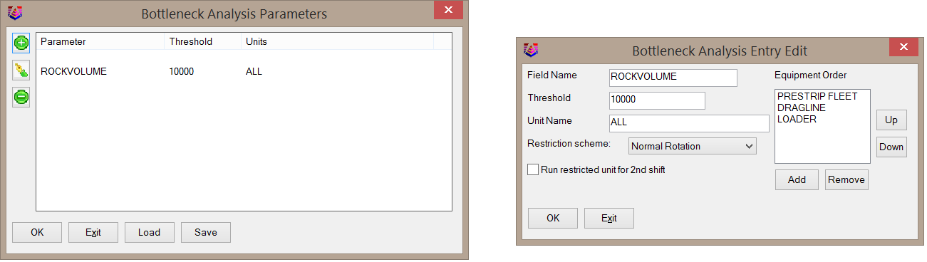
Do Earlier: This button will move the
currently selected bench upwards in the list, causing it to be
mined earlier in the sequence.
Do Later: This button will move the currently selected bench
downwards in the list, causing it to be mined later in the
sequence.
Remove: This button will remove the currently selected bench
from the list, allowing it to be re-assigned to another piece of
equipment.
Remove All: This button will remove all assignments from the
currently selected unit.
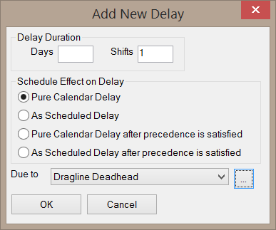
Add Delay: This button will open the dialog shown below,
which controls how delays are handled. A delay will appear in the
Assignment Column as if it were another bench to be mined, and may
be moved up or down in the sequence.
Delay Duration: These values control how long the delay
lasts. In the above example, the equipment will be delayed for a
full shift. Note that partial shift delays are allowed.
Pure Calendar Delay: This option will not force a delay. If
the equipment already has scheduled downtime when the delay is
encountered, additional time will not be taken off.
As Scheduled Delay: This option will force a delay even if
the equipment already has scheduled downtime when the delay is
encountered. The delay will wait until the scheduled downtime is
complete, then the delay will be applied.
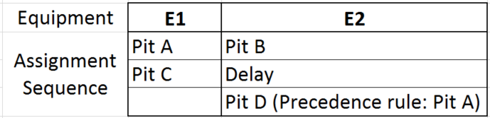
Pure Calendar Delay after precedence is satisfied: This is
similar to a Pure Calendar Delay, but will not attempt to apply the
delay until precedence rules have been satisfied. Consider the
below scenario. Equipment E1 is scheduled to mine Pit A and Pit C.
Equipment E2 is scheduled to mine Pit B and Pit D. A precedence
rule has been created that does not allow Pit D to be mined until
Pit A is complete. A delay of this type is placed on Equipment E2
after Pit B. In this scenario, the finish date of Pit A will first
be calculated, then the delay will be applied. If the equipment
already has scheduled downtime when the delay is encountered,
additional time will not be taken off.
As Scheduled Delay after precedence is satisfied: This
option is similar to a As Scheduled Delay, but will not attempt to
apply the delay until precedence rules have been satisfied.
Consider the below scenario. Equipment E1 is scheduled to mine Pit
A and Pit C. Equipment E2 is scheduled to mine Pit B and Pit D. A
precedence rule has been created that does not allow Pit D to be
mined until Pit A is complete. A delay of this type is placed on
Equipment E2 after Pit B. In this scenario, the finish date of Pit
A will first be calculated, then the delay will be applied. If the
equipment already has scheduled downtime, the delay will be applied
in addition to this downtime.
Due To: This dropdown menu lists the Drawing Event delays in
the Timing Project Manager. The ellipse button will allow you to
define a new Drawing Event.
The Unassigned Column lists all benches that have not yet been
assigned to a piece of equipment.
Assign: This button will assign the currently selected bench
to the currently selected piece of equipment. Multiple benches may
be selected at a time by holding CTRL while clicking or holding
SHIFT while clicking.
Select: This button will select all benches according to the
drop-down menu to the right of this button. If the drop-down menu
is set to NONE, then all benches will be unselected. If the
drop-down menu is set to ALL, then all benches will be selected. If
the drop-down menu is set to Bench 1, then Bench 1 from every pit
in the list will be selected.
Sort: This drop-down list will sort the benches according to
a variety of options.
- Pit, Bench: this option will sort the list in order of
increasing pits, then in order of increasing benches (Pit1-B1;
Pit1-B2; Pit2-B1; Pit2-B2; etc.)
- Bench, Pit: this option will sort the list in order of
increasing bench, then in order of increasing pit number (Pit1-B1;
Pit2-B1; Pit2-B1; Pit2-B2; etc.)
- X-Bench Staircase: this option will sort the benches in a
staircase method according to the number of benches available. A
three-bench scenario will sort the benches in a staircase-fashion
such as
Pit1-B1; Pit2-B1; Pit1-B2;
Pit3-B1; Pit2-B2; Pit1-B3; Pit4-B1; Pit3-B2;
Pit2-B3 etc.
Inv: This checkbox will invert the order of the Unassigned
Column.
Use Precedence: This checkbox will ensure that precedence is
satisfied in the list. For example if Pit1-B1 is assigned to
precede Pit1-B2, toggling this option on will reorder the list so
that Pit1-B1 is listed before Pit1-B2.
Screen Pick: This button will allow selection of the pits
from plan-view in the actual drawing area. When activated, the
Surface Equipment Timing Dialog will disappear and the drawing area
will be visible. The command line will prompt you to click inside
the pit to assign to the currently selected piece of equipment.
Pits/benches that have already been assigned to a piece of
equipment will be filled with a transparent color. Clicking inside
a pit will assign the top available bench in that pit and the pit
will be filled with a transparent color to indicate it has been
selected. Clicking inside the pit a second time will assign the
next available bench and the highlighting color will change to
indicate that the second available bench has been assigned.
Pressing ENTER after selecting the benches will return to the
Surface Equipment Timing dialog. An example of the Screen Pick
method of selection is shown below.
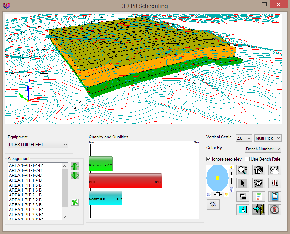
3D Pick: This button will open a new window, as shown below,
to show a 3D view of the available pits and the volumes/qualities
associated with them.
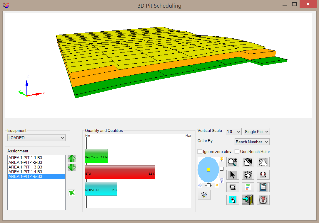
The benches shown in the 3D graphics window will be
shown as flat benches by default. However, benches may be
associated with elevation surfaces to show realistic dimensions via
the Timing Project Manager attribute groups. More information on
this feature is available in the Timing Project Manager article of
the help manual.
Equipment: This drop-down list includes all equipment that
have been added to the main Surface Equipment Timing dialog.
Benches may only be assigned to the currently selected
equipment.
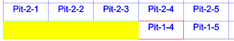
Assignment Column: This list shows all benches that have
been assigned to the currently selected equipment. The benches are
listed in the order they will be mined, from top to bottom. The
green arrows to the right of this list will move the currently
selected bench up and down in the list. The green X to the right of
this list will remove the currently selected bench from the list
and make it available for assignment to another piece of
equipment.
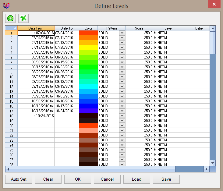
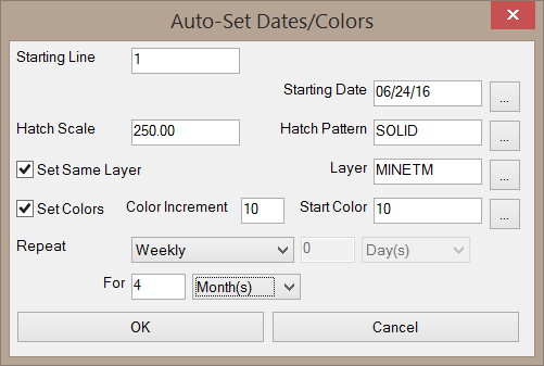
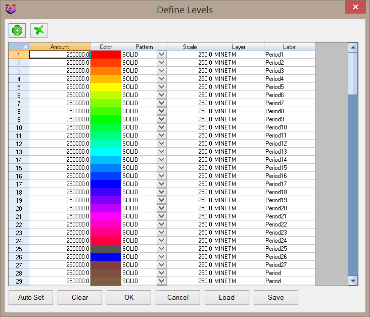
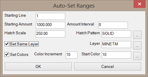
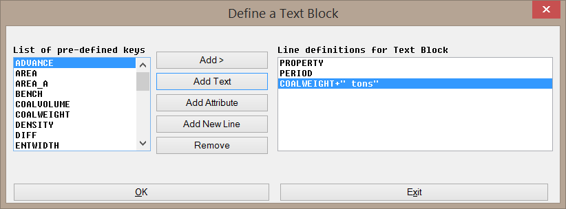
Quantity and Qualities Graph: This graph shows the overall
quantity and qualities of material from all assigned pits. As
benches are assigned to a piece of equipment, this table will
dynamically update. The appearance of this table is controlled with
the Chart Settings icon.
Vertical Scale: This value controls the vertical
exaggeration of the graphics window.
Single Pick/Multi Pick: This drop-down list, just to the
right of the Vertical Scale value, controls how benches are
assigned to equipment. When the Single Pick option is selected,
benches must be added one at a time by double-clicking on each
bench. When the Multi Pick option is selected, multiple pits may be
assigned by double-clicking the first pit in a line to be mined,
then double-clicking the last pit to be mined. Additional lines of
pits may be added with additional double-clicks. Once the
appropriate pits have been selected, they may be assigned to the
equipment by right-clicking the mouse.
Color By: This drop-down list controls how benches are
colored in the graphics window.
When the Bench Number option is selected, all benches of a
particular level will be colored similarly.
When the Grade option is selected, benches will be colored
according to a grade parameter file. The overall quality of the pit
determines the grade categorization, and thus the coloring of the
pit.
Ignore zero elev: This option will toggle the visibility of
surface features at zero elevation in the graphics window.
Use Bench Rules: This option will apply the bench rules to
benches on top and those are assigned to the equipment selected for
each bench in order top to bottom with defined sequence.
Icons: The bottom right of the 3D Pick window dialog
contains several icons. Hovering over each icon will display a
pop-up of the icon's name. These icons are also named in the below
image, listed in order from left to right.
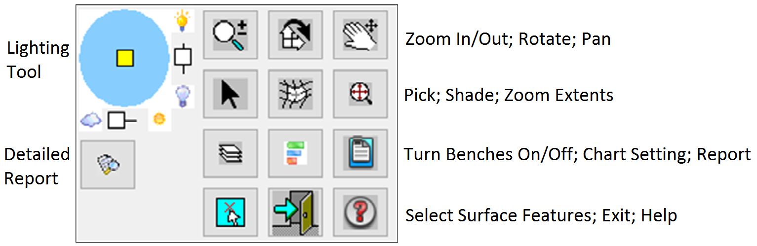
Lighting Tool: This icon controls the
lighting of the graphics window. The yellow square inside the blue
circle represents the position of the light source. Moving this
square will change the shading of the graphics window. The vertical
slide bar to the right of the blue circle controls the intensity of
the light. The horizontal slider bar below the blue circle controls
the amount of light.
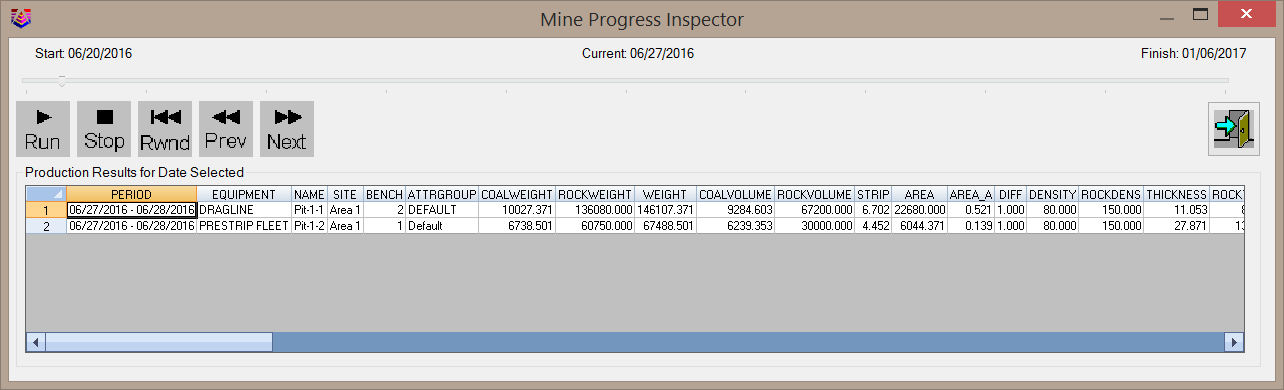
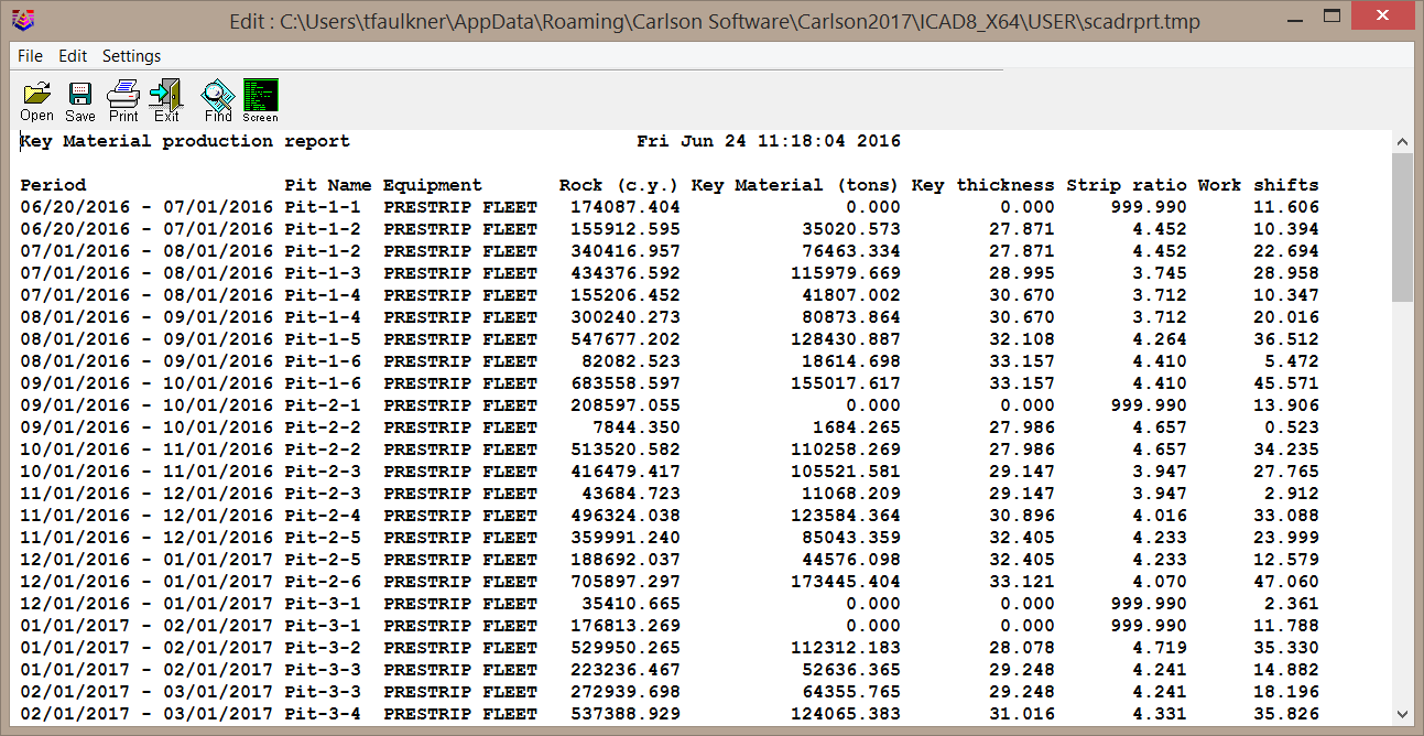
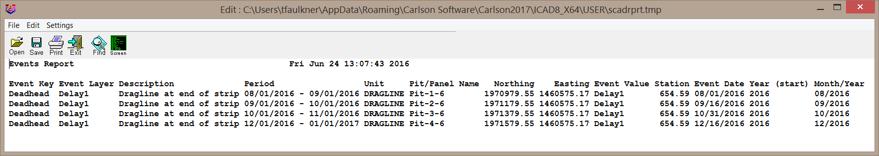
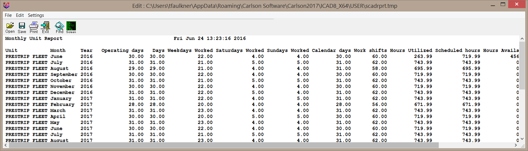
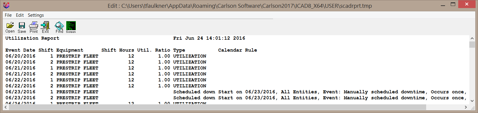
Detailed Report: This icon will open the window shown below,
which gives detailed information about the currently assigned
benches. This window will remain active along with the 3D Pick
dialog.
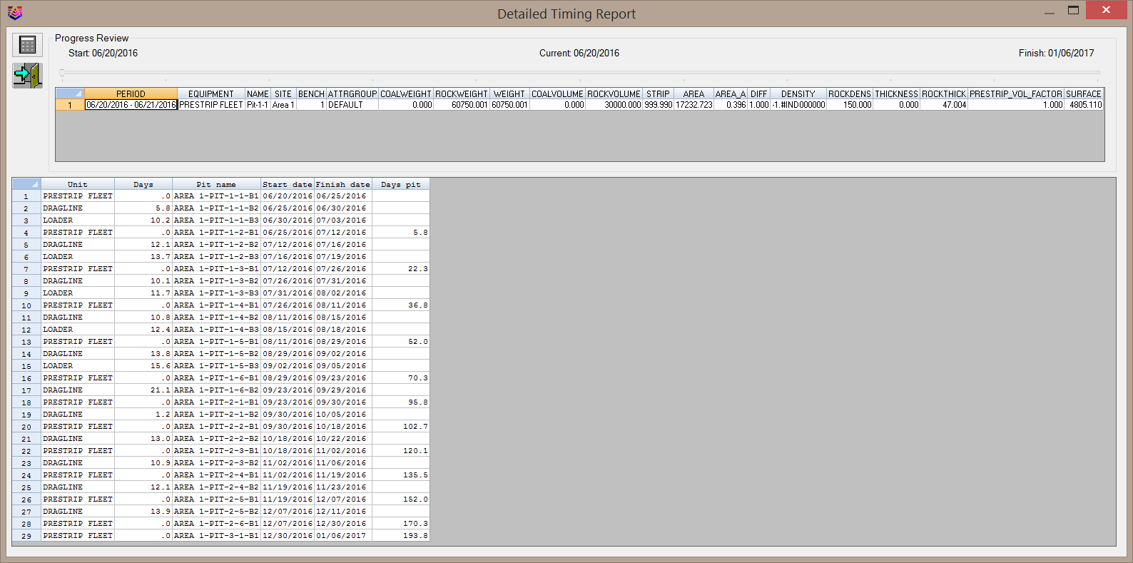
The calculator icon at the top left of the screen
will recalculate the timing results of the currently assigned
benches. This allows additional pits to be added/removed from the
assigned equipment and then quickly recalculate the impact on the
scheduling.
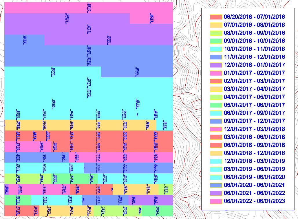
The slider bar at the top of dialog represents the timeline of the
mining progression. Clicking-and-dragging the slider will update
the displayed information.
The spreadsheet report will display benches to be mined in the
currently selected time period.
Zoom In/Out: This icon will change the cursor of the
graphics window to a magnifying glass. When active,
clicking-and-dragging the left mouse button forward or backward
will zoom in or out, respectively.
Rotate: This icon will change the cursor of the
graphics window to show X and Y axes. When active,
clicking-and-dragging the left mouse button will rotate the objects
shown in the graphics window.
Pan: This icon will change the cursor of the graphics window
to a hand. When active, clicking-and-dragging the left mouse button
will pan the objects shown in the graphics window.
Pick: This icon will change the cursor of the graphics
window to a standard, black cursor. When active, double-clicking
benches in the graphics window will assign them to the currently
selected piece of equipment.
Shade: This icon will toggle the shading of pits in the
graphics window between a wireframe view and a full color-filled
view.
Zoom Extents: This icon will reset the zoom of the graphics
window so that all entities are visible.
Turn Benches On/Off: This icon will open the Bench
Sequencing dialog, shown below. This is intended to assist with
sequencing when using the Single Pick option of selecting benches.
When a bench is selected for mining, other benches will be
automatically selected based on these bench rules. Note that the
Use Bench Rules checkbox must be selected to use these rules. Note
that in order to use the Bench Rules, pits must be oriented in the
N-E-S-W directions. If the pits are not naturally oriented this
way, the Twist Screen command may be used (prior to executing the
Surface Equipment Timing command) to align the pits in the N-E-S-W
directions.
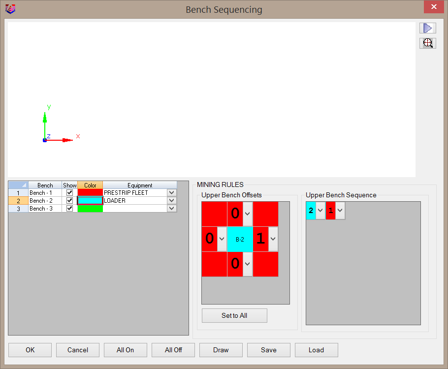
The Graphics window at the top of this dialog will show
an example of the bench rules to be applied.
The List of Benches on the left side of this dialog controls
various options for the benches.
Bench Column: This column lists the benches in order from
top to bottom.
Show Column: This column controls if benches are shown in
the graphics window.
Color Column: This column controls the color of each bench.
Double-clicking one of the color cells will open the CAD color
palette for color selection.
Equipment Column: This column controls which piece of
equipment the bench will be assigned to. If no equipment is
specified, all benches will be assigned to the current equipment
selected on the 3D pick dialog.
The Mining Rules on the right side of this dialog control the
automatic sequencing of the benches.
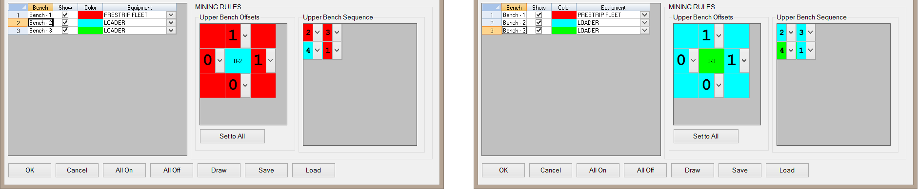
Upper Bench Offsets: This graphic controls how many benches
should be developed in addition to the bench that is actually
selected in the 3D Pick dialog. The center square represents the
bench that is selected in the 3D pick window. The numbers on each
side of this square control how many upper-level benches must be
sequenced in addition to the selected bench. In the above image,
anytime a bench on level-2 is selected for sequencing, the bench on
level-1 just to the east will also be sequenced. These benches will
be assigned to the equipment specified in the Equipment Column.
Upper Bench Sequence: This graphic controls actual
sequencing of the automatically sequenced benches. In the above
image, the upper bench (red) will be sequenced first, then the
level 2 bench will be developed.
Set to All: This button will apply the current bench
sequencing rule to all other benches.
All On: This button will turn on all benches in the graphics
window.
All Off: This button will turn off all benches in the
graphics window.
Draw: This button will draw a preview of the selection in
CAD. Picking a bench will fill in that bench with a yellow hatch.
All other benches to be automatically sequenced along with this
bench will be outlined with the same Bench Color. In the below
example, Pit 1-3 Bench 2 has been picked for scheduling, and Pit
1-4 Bench 1 has been outlined to show that it will be automatically
sequenced.
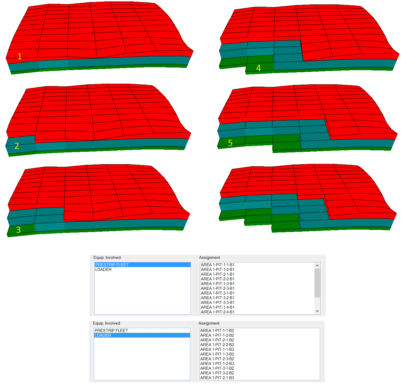
Bench Sequence Rules Example:
The below images show the bench rules for a 3-bench example. In
this example, whenever a level-2 bench is selected, up to 3 level-1
benches will also be sequenced. Whenever a level-3 bench is
selected, up to 3 level-2 benches will also be sequenced. These
rules compound, meaning that whenever a level 3-bench is selected,
up to 8 level-1 benches may also be sequenced.
Using these bench rules, 5 benches were manually
picked as shown below. The yellow number indicates the benches that
was actually selected; all other benches were automatically
assigned to the appropriate equipment. The final sequence applied
to each piece of equipment is also shown below this progression.
This allows a total of 26 benches to be sequenced by manually
selecting only 5 benches. This can save tremendous amounts of time
when working with multi-bench pits.
Chart Settings: This icon will open the chart settings
dialog, shown below. These settings will determine the appearance
of the Quantity and Qualities chart shown to the right of the
dialog.
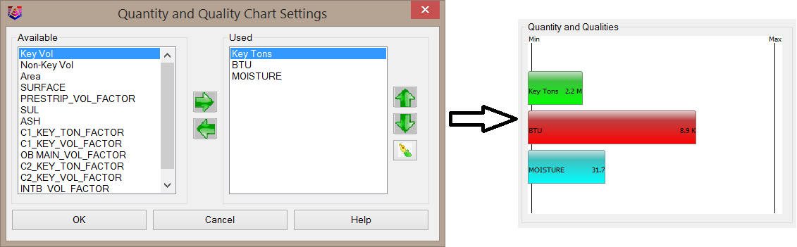
This dialog contains two columns: Available and
Used. Only items in the Used Column will be shown in the Quantity
and Qualities chart. Items may be moved between the two columns by
selecting the item and clicking one of the green arrows between the
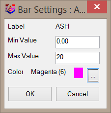
two columns. When an item is first moved to the Used Column, the
below dialog will appear to control that item's appearance on the
chart, including minimum value to display, maximum value to
display, and color.
To the right of the Used Column are three icons.
The green arrows can be used to move the currently selected item up
and down in the list. The green ink quill can be used to edit the
appearance of the currently selected item.
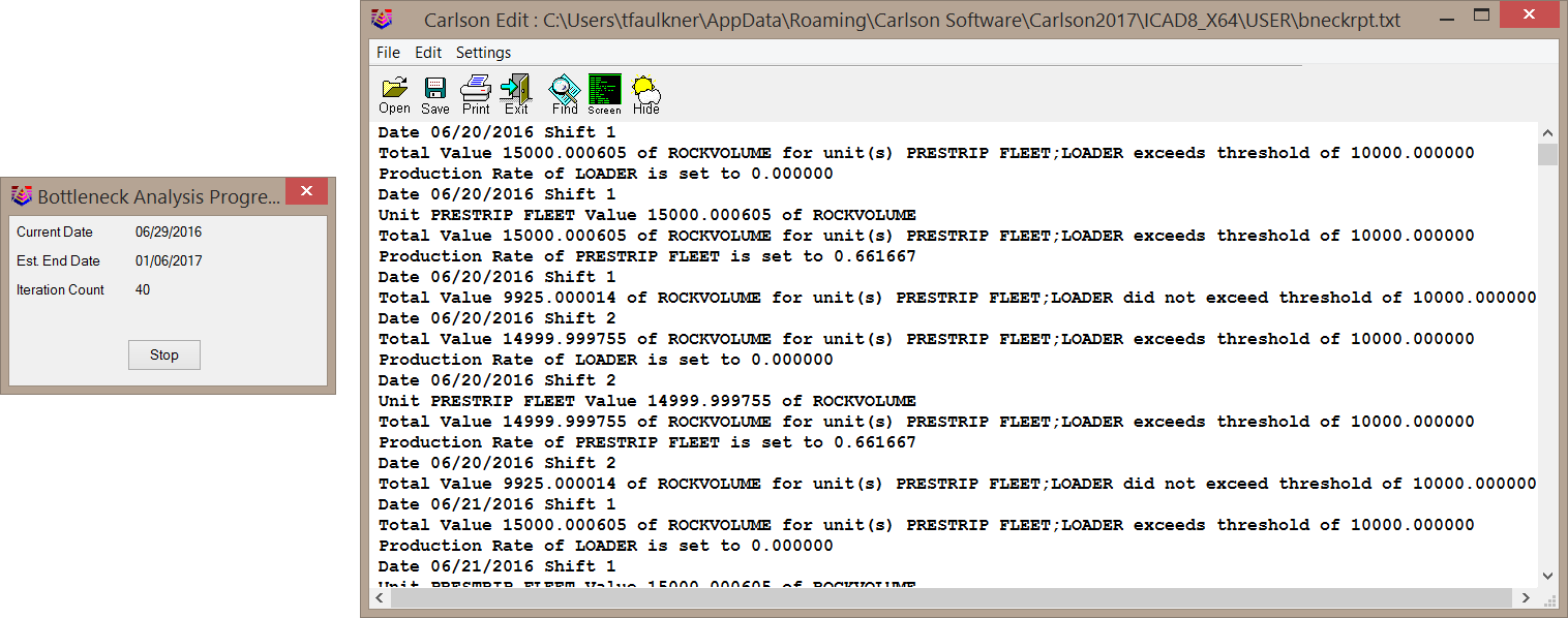
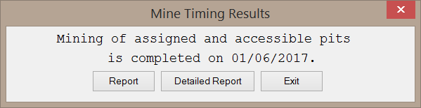
This button will continue with the Surface Equipment
Timing command to calculate the amount of time required to mine the
assigned benches. This function is discussed later in this section
of the help manual.
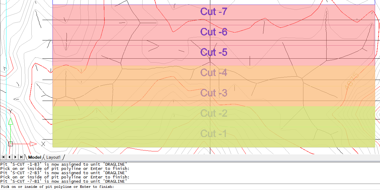
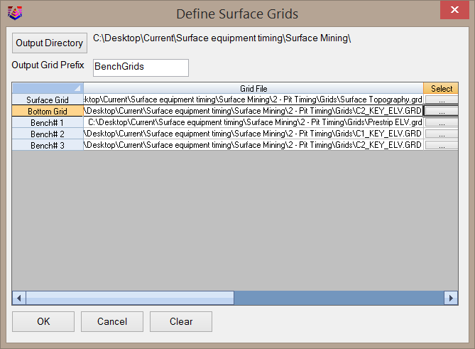
Select Surface Features: This button will allow you to
select CAD linework to add to the 3D viewer window. The below image
shows the dialog with contour lines and breaklines added to the 3d
viewer. Entities may be removed from the 3D viewer window by
clicking this icon again and end the selection without actually
selecting any CAD linework.
Exit: This icon will exit the 3D Pick
dialog.
Help: This icon will open the help manual you're currently
reading!
Additional scheduling options are listed below the Equip. Involved,
Assignment, and Unassigned Columns.