In this tutorial, we'll layout the structure and pipes for the stormwater drainage and analyze the flow for a portion of a site. We'll use the tools to automatically calculate the drainage and runoff coefficients. These automated methods require setup of a surface and runoff regions. Alternatively, these tools can be skipped in which case the drainage areas and runoff coefficients for the inlets can be entered manually into the sewer network.
From the File menu, choose Open and select EXAMPLE3.dwg from the Carlson Work folder (e.g. C:\Carlson Projects\EXAMPLE3.dwg).
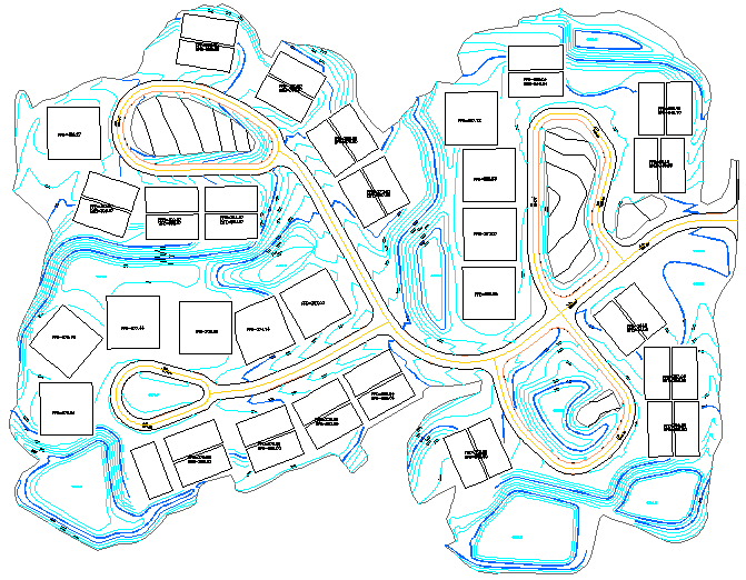
The drawing entities for the design surface that we will use to model drainage have already been prepared. These entities consist of design contours, elevated pad perimeter polylines, spot elevations and 3D polylines for the road centerlines and face of curbs.
To model the drainage, the program can use either triangulation or grid surfaces. For this example, triangulation is used so that the flow can follow the edges of the road. In general, triangulation is needed for surfaces with breaklines and grids are useful for surfaces defined by contours alone.
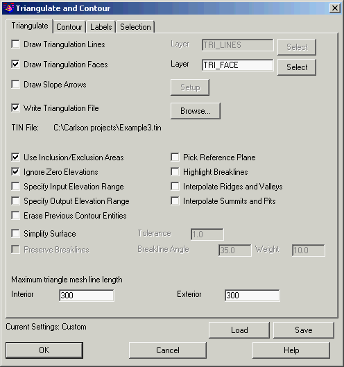
Run the Triangulate & Contour command from the Surface menu. In the dialog, go to the Contour tab and turn off Draw Contours. Then in the Triangulate tab, turn on Draw Triangulation Faces, Write Triangulation File, Use Inclusion/Exclusion Areas and Ignore Zero Elevations. Pick the Browse button and set the file name as Example3.tin. Then pick OK.
At the command line, the program will prompt for the inclusion and exclusion perimeters. Pick the perimeter polyline for the inclusion and nothing for exclusion. Next, for the select objects to triangulate, type All and press Enter.
Select the Inclusion perimeter
polylines or ENTER for none.
Select objects: pick the
perimeter polyline
Select objects:
press Enter
Select the Exclusion perimeter
polylines or ENTER for none.
Select objects: press
Enter
Select the points and breaklines
to Triangulate.
Select objects: All
Select objects:
press Enter
This step is optional to verify that the surface is good by checking for bad elevation data points and that the surface follows the data points.
With the triangulation drawn as 3D Faces, run the 3D Viewer Window command in the View menu. At the command line, it will prompt to select the objects to view. Type All and press Enter.
Select all entities for the
scene.
Select objects: All
Select objects:
press Enter
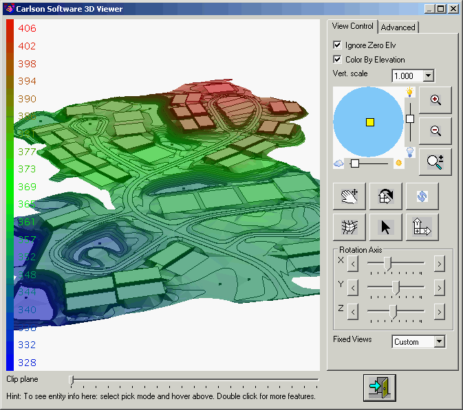
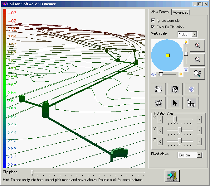
In the 3D Viewer dialog, move the pointer near the center of the graphic and the cursor will change to an X/Y symbol which is the X/Y axis rotation mode. Click down the left mouse button and drag down to rotate the site to a good viewing angle. Then move the pointer near the edge of the graphic and the cursor will change to a Z symbol which is the Z axis rotation mode. Click down the left mouse button and drag around to rotate the pile. To fill in the triangulation faces, pick the Shade icon.

You can also choose the Color By Elevation toggle for better viewing of the elevation range.
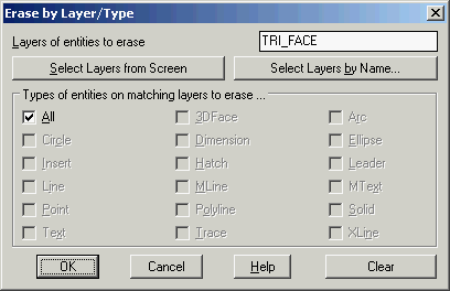
The surface looks right in the 3D Viewer. The site has a slope from the top road circle down towards the detention ponds at the bottom. Close the 3D Viewer by choosing the Exit Door button. We don't need the 3D Faces anymore. Let's delete them by running Erase By Layer in the Edit menu. Choose the Select Layers From Screen and pick any 3D Face. Then pick the OK button.
This step sets up layers that are assigned Rational Method runoff coefficients and applied to closed polylines on the specified layers. The runoff coefficients are the C-Factors in the Rational Equation Q = C*I*A.
Q is flow, I is rainfall intensity and A is area. The runoff polyline areas use region logic where a polyline inside another on the same layer is used as an exclusion. A limitation is that polylines on the same layer must not intersect each other. For polylines on different layers, there can be polylines within other polylines and for any given point; the smallest enclosing polyline is used to determine the runoff coefficient.
In this example, the site perimeter polyline is on the Regions layer, the building pads are on the Pads layer and the edge of pavement polylines are on the Roads layer. All these polylines are already closed polylines. So we're ready to assign the runoff coefficients to the layers. Run Define Watershed Layers in the Watershed menu. Begin with an empty dialog by deleting any existing layers in the table. Select the Add button.
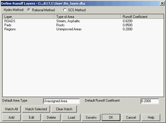
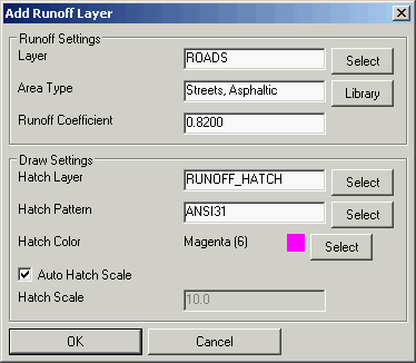
Let's add the road layer first. Use the Select button next to the Layer field and select the layer name ROADS from the list or screen pick a road polyline. Next choose the Library button and select Streets, Asphaltic from the list. Under the Draw Settings, set the Hatch Color to Magenta. When the dialog is set as shown, pick OK.
Repeat the Add function for the Pads layer and set the runoff to Roofs and the color to Red. Again, repeat add for the Regions layer and set the runoff to Unimproved Areas and the color to Green.
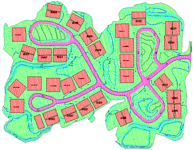
From the main dialog, pick the Hatch All which gives a visual check of the runoff coefficient areas. The areas within the buildings are inside both the Region and Pads polylines and the Pads govern because they are the smaller area. Likewise the road areas are governed by the Roads layer and road interior islands are not counted for Roads because the interior Roads polyline acts as an exclusion perimeter. The rest of the area is set to the Regions layer.
With the three layers defined, click OK from the main dialog.
We don't need to keep the runoff hatches. Let's delete them by running Erase By Layer in the Edit menu. Choose the Select Layers From Screen and pick any hatch to get the RUNOFF_HATCH layer. Then pick the OK button.
From the Watershed menu, pick Watershed Analysis and when prompted for the surface file, choose Example3.tin. The program dialog docks on the left side of the drawing.
Before processing the watersheds, set the Rainfall to 1 inch. The program uses the runoff volume calculated from the rainfall depth and drainage areas to figure when the runoff is enough for the flow to go through a low point. If the rainfall depth is set to zero, then the flow lines will stop at every low point or dimple in the surface. At this point, we have not defined our storm event to know the actual rainfall depth. If we did get the storm rainfall depth, we could enter it. For now we're just using Watershed Analysis to give a general idea of the watershed areas and runoff flow lines.
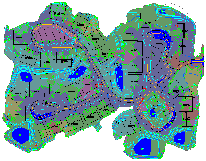
First, go to the Draw tab and turn on Fill Watershed Areas, Sink Locations and Pond Areas.
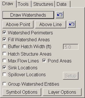
Now pick the Draw Watersheds button. Each watershed area is drawn with a closed polyline and solid filled with different colors. Also, for each watershed the sink (lowest point) is drawn with a solid circle symbol. The areas covered by ponding are drawn as solid blue hatches. The depth and size of the pond areas is determined by the runoff volume. In many places, the pond areas are inside the detention pond structures. In a few places, the ponds are at low points in the road which indicate areas that we need to add storm sewer inlets.
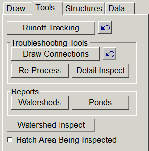
To navigate around the watershed display, move the pointer into the graphic view and use the middle button of the wheel mouse, if you have one, to pan and zoom. If you don't have a wheel mouse, then use the top toolbar icons of the Watershed Analysis dialog to zoom and pan. When you are done inspecting the watersheds, pick the back arrow (shown below) next to the Draw Watershed button to erase all the watershed entities.

Next, choose the Runoff Tracking button under the Tools
tab.
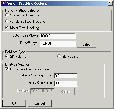
In the options dialog, choose Major Flow Tracking that draws flow
lines only when the drainage area for the flow line is greater than
the specified area. Then choose the 2D Polyline type and the Draw
Flow Direction Arrow to use a flow linetype with arrows showing the
flow direction.
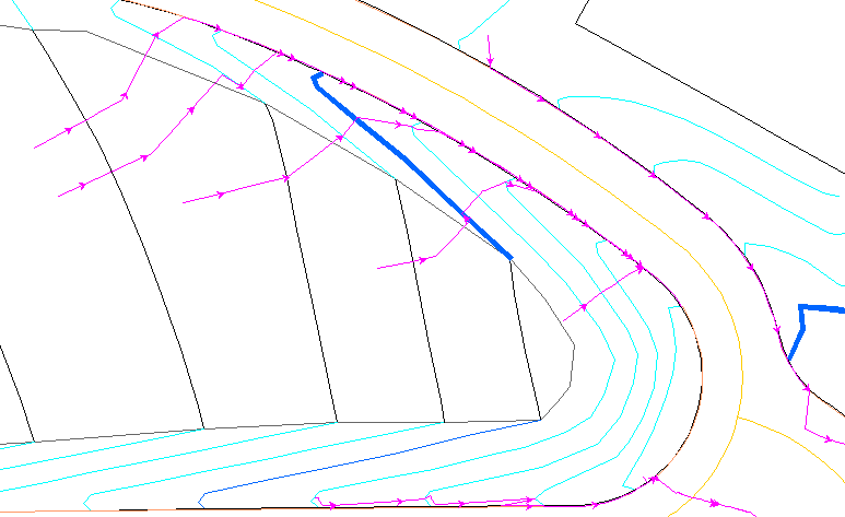
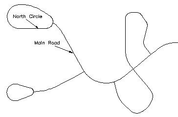
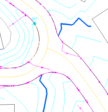
Use the zoom and pan methods to inspect the runoff flow lines. This graphic shows the flow lines coming off the road circle at the top of the site and following the curbs. We're going to leave the runoff flow lines on the drawing to help guide the placement of inlets. Click Exit to end Watershed Analysis.
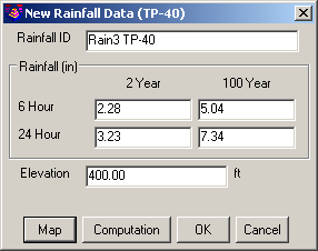
To setup the storm event to apply with this site, run Rainfall Library under the Sewer Network Libraries flyout in the Network menu. This command keeps a list of different storm events that you can use for different locations and requirements. Let's add a storm by picking the New button. There are six types of rainfall definitions. For this example, select the Rainfall Total (TP-40) method. In the New Rainfall dialog for the TP-40 method, fill in a name for the Rainfall ID, the rainfall amounts for the 2 and 100 year storms for 6 and 24 hours, and the average elevation for the site.
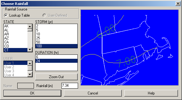
You can use the Map button to show the TP-40 rainfall maps for the different storms. And if you pick on the map display, the program will interpolate the rainfall from the maps. In this case, south central CT was picked.
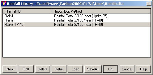
Click OK on the New Rainfall dialog and then pick OK on the Rainfall Library dialog to save the changes.
In preparation to align the inlet symbols with the road centerlines, we need to create centerline files (.cl) for the roads. From the Centerline menu of the Civil Design or Survey modules, choose Polyline To Centerline File. In the file selection dialog, enter a name of North.cl. Then enter a starting station of 0, pick the road centerline for the loop road at the top of the site and press Enter at the end of the station list.
Beginning Station
<0+00>: press
Enter
Polyline should have been drawn in
direction of increasing stations.
Select polyline that represents centerline: pick the north loop road
centerline
Press ENTER to continue.
press Enter
Repeat Polyline To Centerline File. For the file name, enter Main.cl. Enter a starting station of 0 and pick the main road centerline.
The storm sewer network structures and pipes are stored in a .SEW file. Once a .SEW file is set as current, the program will continue to automatically use that file. To start a new sewer network, run Set Sewer File under the Sewer Network Setup flyout of the Network menu. In the file selection dialog, choose the New tab and enter a file name of Example3.sew.
The sewer network also works with a current surface model that
is used for the default rim elevations, reporting pipe cover and
calculating inlet drainage areas. To set the current surface, run
the Set Surface File under the Sewer Network Setup flyout of the
Network menu. In the file selection dialog, choose our Example3.tin
file.
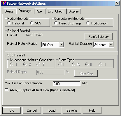
Before creating the sewer network set defaults in Network >
Sewer Network Setup > Sewer Network Settings. In the Drainage
tab click Library to set the Rainfall to Rain3 TP-40 created
earlier and a return period of 100 years.
Before starting the layout, set the object snap (osnap) to nearest (nea) to use for locating the inlets along the curb polylines. Under the Settings menu, run Aperture-Object Snap and turn on only the Nearest snap mode.
Now we're ready to layout the inlets and pipes. Let's work on the drainage for the roads of the north loop and the main road and run this flow to an outlet in the central pond.
Run Create Sewer Structure from the Network menu. The first prompt is to select from three methods to locate the inlets. Press Enter to choose the default method of screen pick. Next the inlet location is picked. Decide where to put the inlet. You can look at the runoff flow lines and place the inlet to capture these flows. When you have a place for the inlet, zoom in very close so that you can see the curb line.
NOTE: Be sure to pick the bottom, inside curb polyline and not the top of curb. Otherwise, the routine to find the drainage area from the surface model will not capture flow along the curb.
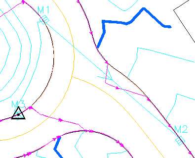
If you have a wheel-mouse, use the wheel to do the zoom in. Otherwise you can use the zoom toolbar or type 'z at the command prompt. After zooming in, pick a point along the curb polyline using the nearest snap to get right on the polyline. In this case, the first inlet will be on the inside curb of the north loop near the intersection as shown with the M1 symbol.
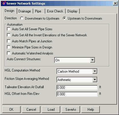
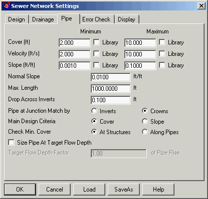
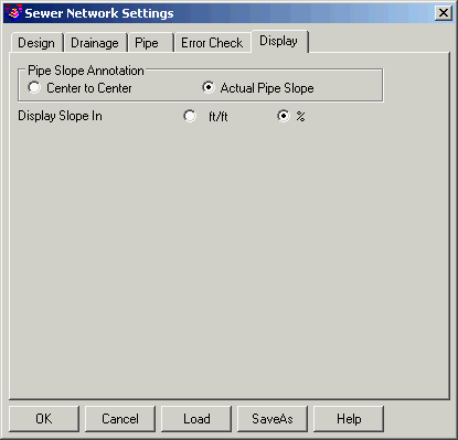
After this first inlet location is picked, the sewer network dialog is docked on the left side of the drawing. Next choose the Settings button and, on the Design tab, set the Direction to Upstream To Downstream, and uncheck the Minimize Pope Sizes in Design option. The Pipe Settings allow you to configure your design parameters. Select the Pipe tab, and change the Minimum Cover and Velocity to 2.0, Maximum Cover and Velocity to 10.0, and the Drop Across Inverts to 0.1. Now select the Display tab, and set the Display Slope In to %. Next select the Drainage tab and pick the Rainfall Library button and pick the rainfall event set in Step 6. Let's go with defaults for the rest. Pick the OK button.
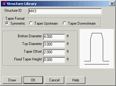
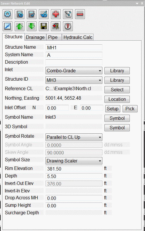
Now let's work on the structure settings. Pick the Library button next to the Structure ID field. This function brings up a list of the available structures as defined in the library. There are three types of structures: box, circular and outfall. You can add your own structures to the library. For this example, use MH3. To check the dimensions for this structure, pick the Edit button. These dimensions are used for hydraulic calculations as well as drawing the structure in the profile and 3D views. Click OK from the Edit dialog and then highlight MH3 from the library list and pick OK.
Next, pick the Library button next to the Inlet field. This function shows the inlets defined in the inlet library. There are four types of inlets: slotted, curb, grate and curb/grate combo. Inlets can also be defined as located on-grade along the road or at a sag location. Like the structure library, you can add to and edit the inlet library. For this inlet, choose the Combo-Grade from the list and pick OK.
Next, pick the Select button next to the Reference CL label, select by Centerline File, and select North.cl for the centerline. This centerline can be used to align the inlet symbol. In the Symbol Rotate field, choose Parallel To CL Up.
The last change for the structure tab is to set the Depth to 5.5. After making these changes, your dialog should match the settings as shown. Pick the Apply button to save the changes and you should see the plan view symbol for the inlet change to a grate symbol.
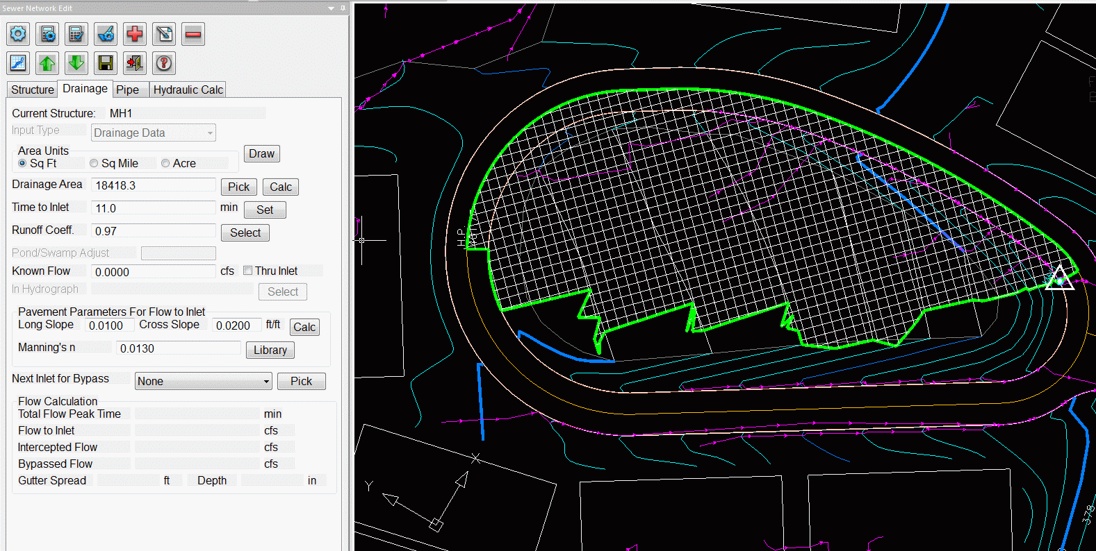
Now move onto the Drainage tab. Here the drainage area, time of concentration, runoff coefficient and pavement parameters are set for the inlet. You can manually enter in or have the program calculate these values. With the Pick button, you can select a drainage polyline perimeter and the program will calculate the area and the weighted average runoff coefficient from the runoff layers if defined. In this example, use the Calc button to calculate all the parameters from the surface model. The first time that Calc is called, the program takes time to calculate the triangulation flows. Then the values are filled in and the drainage area is hatched in plan view. The Time To Inlet comes from the max flow line within the drainage area and accounts for the surface slopes along the path. The Runoff Coefficient is calculated as the weighted average of the runoff sub-areas within the drainage using the runoff layers that we defined in the Define Runoff Layers command. Notice how the drainage area for M1 starts from the road high point and follows the crown of the road to the inlet. In the Pavement Parameters section, the Calc button will calculate the Pavement slopes from the surface aligned by the reference CL at the inlet location.
We're done for now with this first inlet. To add the next inlet, pick the Add button from the Structure Actions row. Pick a position along the right side curb polyline of the main road near the intersection as shown here (M2). Again, you may need to zoom in to be sure to snap onto the curb polyline.
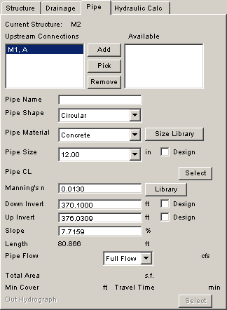
Go to the Structure tab for M2 and change the Reference CL to Main.cl. Then go to the Drainage tab and pick Calc which fills out all the drainage values. Next select the Pipe tab. The program lists all the used and available structures for a pipe connection to the current structure. By default, a connection is made to the nearest structure as long as it's within the maximum pipe length as defined under Settings. In the dialog, set the Down Invert to 370.1. Switch back to the Structure tab and set the Invert-Out as 370.0.
To add the next inlet, pick the Add button. Then pick a position along the inside North loop curb polyline to the left of the intersection as shown here (M3).
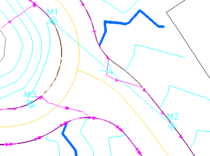
A pipe is automatically connected to the nearest structure M1. But for this network, we don't want M3 to connect to M1. Instead, we're going to start new branch with M3. So go to the Pipe tab highlight the Upstream Connection list for M1 and pick the Remove button. On the Structure tab for M3, set the depth to 5.5. On the Drainage tab, pick Calc.
Now we're ready for the next inlet. Pick the Add button in the Structure Actions row and screen pick the position along the main road across from M2 as shown here (M4).
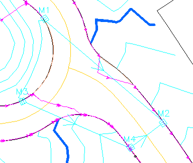
This inlet is on the other side of the road and the symbol is rotated the wrong way. To fix this, go to the Structure tab and change the Symbol Rotate to Parallel To CL Down and pick Apply to update the drawing. Also, change the Invert-Out to 371. Next go to the Drainage tab and pick the Calc button. Again the pipe connection defaulted to the nearest structure of M2. Instead we want the connections to go from M3 to M4 to M2. Under the Pipe tab, highlight the Upstream Connection for M2 and pick Remove. Then highlight the Available structure of M3 and pick Add. For the pipe parameters, change the Down Invert to 371.1. Then go back to the Structure tab and set the Invert-Out to 371.0.
To create the pipe from M4 to M2, pick the Edit button in the Structure Actions row. Then pick on the M2 label or symbol to edit M2. From the Pipe tab, highlight M4 from the Available list and pick Add.
Now let's add the next inlet. Pick the Add button in the Structure Actions row and pick a position further down the main road from M4 as shown here (M5).
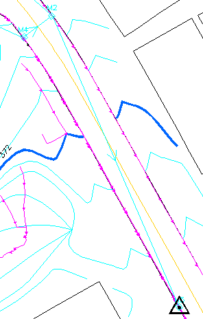
Under the Structure tab, change the Depth to 4.5 and set Symbol Rotate to Parallel To CL Down. Under the Drainage tab, pick Calc. Again we want to remove the default pipe connection since M5 will be the start of a new branch. Go to the Pipe tab, highlight the connection listed and pick Remove.
We have one more inlet to add. Pick the Add button and pick along the curb on the other side of the main road from M5. See M6 in the graphic here.
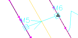
Under the Structure tab, set the Symbol Rotate to Parallel To CL Up to flip the symbol around. Under the Drainage tab, pick Calc. Under the pipe tab, add a connection to M2.
For the last structure, pick the Add button and pick on the 356 contour in the pond to the right of M6.
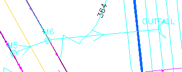
In the Structure tab, change the Structure Name to Outfall, set the Structure ID to Outfall-Wall1 and change the Depth to 4.0. In the Pipe tab, set the Down Invert to 352.0.
The initial sewer network layout is done. Pick the Close button and if prompted whether to Save Change, choose Yes.
The network flow can be analyzed in the Edit Sewer Structure and SpreadSheet Sewer Editor commands. For this example, we'll use Edit Sewer Structure. Either choose this command from the Network menu or double-click on any sewer network label. The same docked dialog from Create Sewer Structure is used. Under the Settings button, and the Drainage tab, choose Period of 50 Year and Duration of 24 Hours. Then pick OK to exit Settings.
Next, pick the Analyze button which runs the selected storm event through the system. If any of our design parameters are exceeded as specified under Settings, the program displays a report. Here's the report for our first Analysis run.
Network Design Warnings

 1 Pipe Slope   : 11.867 %, Max. pipe slope is 10.000 %      From OUTFALL, A to M6, A

 2 Pipe Velocity: 1.294 ft/s, Min. velocity is 2.000 ft/s    From M2, A to M1, A

 3 Pipe Velocity: 1.382 ft/s, Min. velocity is 2.000 ft/s    From M4, A to M3, A

 4 Pipe Velocity: 0.502 ft/s, Min. velocity is 2.000 ft/s    From M6, A to M5, A

 5 Pipe Velocity: 13.353 ft/s, Max. velocity is 10.000 ft/s  From OUTFALL, A to M6, A
Let's take care of warning #1 for the pipe slope. Choose the Edit button on the Structure Actions row and pick the Outfall label or symbol to edit the Outfall structure. To reduce the pipe slope from M6 to Outfall while keeping the upstream pipe slopes, we will create a step-up at M6. Go to the Pipe tab and change the Up Invert to 356.0. This changes the Invert-Out at M6 while holding the Invert-In at M6.
Pick the Analyze button again. The warning report should only have the flow velocity warnings if any. Exit the report if it comes up. The flow velocity warnings can be resolved by resizing pipes and setting inverts which we will do later. Now let's review the flow results from the dialog.
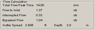
From the Outfall structure, pick the Up button to move up to M6. From the Drainage tab, the flow results are displayed in the Flow Calculation section. The Flow To Inlet is calculated by the Rational Method using the Drainage Area, Time Of Concentration and Runoff Coefficient for this inlet. The Intercepted Flow, Bypassed Flow, Gutter Spread and Gutter Depth are calculated from the inlet dimensions using formulas from HEC-22. These values can be used to determine whether you have the right inlet structure to capture the flow.
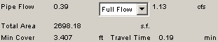
Switch to the Pipe tab. The flow, area and cover are displayed for the pipe connection currently highlighted from the Upstream Connections list. The Total Flow is the accumulated flow for the current pipe. The Total Area reports the accumulated drainage areas for all the inlets coming into this pipe. The Min Cover is calculated using the surface model to the top of the pipe.
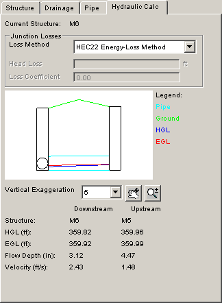
Switch to the Hydraulic Calc tab which shows a graphic of the pipe structure, ground surface, hydraulic grade line (HGL) and energy grade line (EGL), along with the HGL and EGL elevations, Flow Depth and Flow Velocity at the pipe upstream and downstream connections.
You can go to other structures to check the flow values for them or use the Report Sewer Network to review the values in a report view. For our storm event, many of the pipes can be resized. For example, the 12" pipe from M5 to M6 has only 3" flow depth. To resize the pipes, you can go to the Pipe tab and change the Pipe Size. The program can also automatically size the pipes based on the flow. To size specific pipes, go to the Pipe tab and pick on the Design toggle next to the Pipe Size field. Then run pick the Design button at the top of the dialog and the program will run a flow analysis and set the pipe size for these pipes marked for Design. To have the program size all the pipes, choose Auto Set All Pipe Sizes in the Settings dialog and then pick the Design button.
For this example, let's have the program assign all the pipe sizes. Pick the Settings button. Turn on Auto Set All Pipe Sizes and Minimize Pipe Size In Design. Then pick OK. The pipes are resized to match the flow. Pick on the Pipe and Hydraulic tabs to see the changes. Pipes that can change would change and the different pipe sizes that the program uses are defined in the Pipe Size Library.
After the pipe sizing, there are likely a few lingering flow velocity warnings. Experiment with the flow velocity by adjusting invert elevations of the affected pipe(s) in your network. Pick the Structure Action button of Edit and pick the structure whose invert elevations need to be modified.
Now run Analyze function which should now complete without any warnings. Pick the Apply button to save the results and then pick Close.
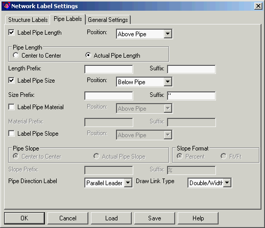
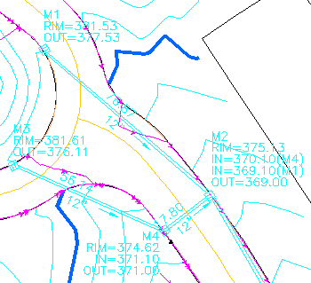
At this point, the sewer network labels are only showing the inlet name and pipe direction arrow. To change the label format, run Plan View Label Settings in the Sewer Network Setup flyout of the Network menu. In the settings dialog, under the Structure Labels tab, Add the Structure Name, Rim Elevation, Invert-In and Invert-Out labels to the Used Labels category. Under the Pipe Labels tab, turn on Label Pipe Length and Label Pipe Size. For Label Pipe Size, set the Position as Below Pipe. Also set Pipe Direction Label to Parallel Leader and Draw Link Type to Double/Width.
The sewer labels are linked to the sewer network definition so that any change to the sewer network updates the labels. If you want to explicitly update the sewer labels, run the Draw Sewer Network > Plan View command.
When sewer labels overlap other drawing entities, you can use the Move Sewer Labels command. Let's run this command and move the M4 label to the left of the inlet.
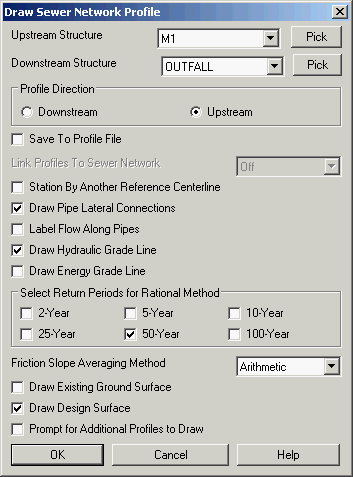
To create a profile for the sewer network, run the Draw Sewer Network > Profile command from the Network menu. In the options dialog, set the upstream structure to M1 and the downstream to Outfall. Also turn on Draw Pipe Lateral Connections, Draw Hydraulic Grade Line and Draw Design Surface. When the setting match the dialog shown here, pick OK.
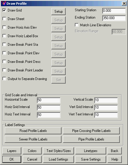
Next, select Example3.tin for the Design Surface File To Read file selection dialog. Then the Draw Sewer Profile program is started. In the Draw Sewer Profile dialog, set the Horizontal Scale and Intervals to 50 and the Vertical Scale and Intervals to 10. Then pick OK.
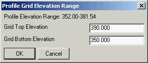
The next dialog prompts for the elevation range for the profile. The elevations default to fit the profile. So just pick OK.
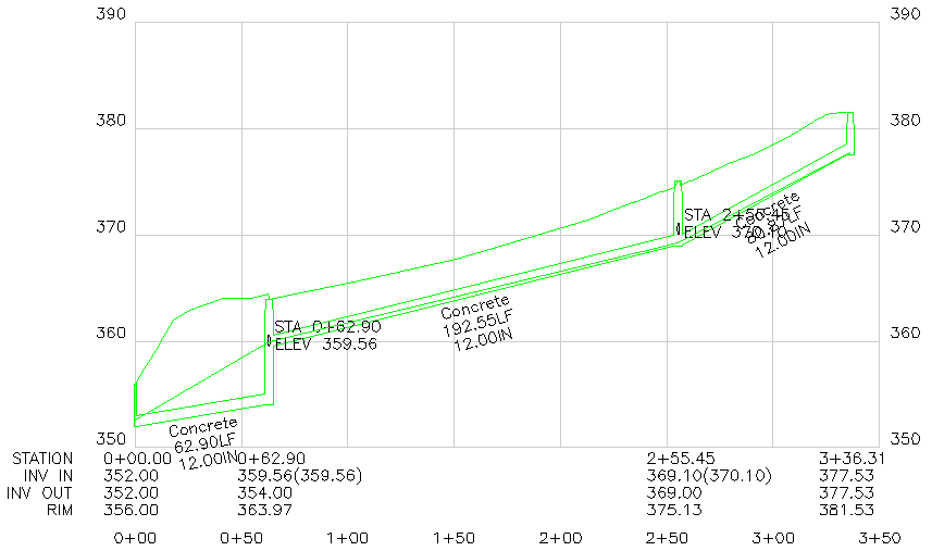
Now there's a prompt to pick the location to draw the profile. First, zoom out to a clear space in the drawing. Then pick the lower left point for the profile. Some of the pipe labels are longer than the pipe segments, and the program prompts whether to draw the labels. Enter Y for yes.
Pick Starting Point for Grid <0.00,0.00>: pick the lower left profile grid point
Next, let's draw the sewer network in 3D. Run the Draw Sewer Network > 3D Faces command in the Network menu. This command draws the structures and pipes as 3D Faces. At the command line, press Enter to use the default layer for the 3D Faces. That's all the prompts for this command.
Enter the layer name [SWRNET3D]: press Enter
To view the 3D Faces, run the 3D Viewer Window command from the View menu. At the select objects prompt, type All and press Enter. Then click and drag the mouse to rotate the view to a good viewing angle as described under the Check Surface step. When done inspecting, exit the viewer by picking the Exit Door button.
Finally, let's check out the reports available under the Report Sewer Network command in the Network menu.
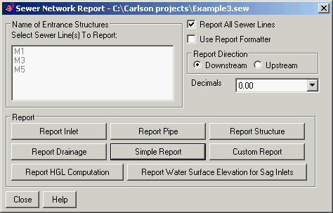
In the Sewer Network Report dialog, you can choose which sewer runs to report and the types of reports to produce. The Report Formatter option allows you to customize which fields to include in the reports and supports outputting the reports to MS Excel and databases. There are specific reports for Inlets, Pipes, Structures and Drainage areas. Let's run the Simple Report to get the summary of our system.
Sewer Network File:            C:\Carlson Projects\example3.sew

Ground Surface File:           C:\Carlson Projects\Example3.tin

Design Method:                 Peak Discharge Calculation

Hydro Method:                  Rational Method

Rainfall ID:                   Rain3 TP-40

Return Period:                 50-Year

Duration:                      24-Hour


System A

Sewer Line From M1 To OUTFALL (Upstream to Downstream)


Name         Station    Invert-In     Invert-Out   Rim Elev       Area(SF)       Flow Depth(in)

             Distance   Slope(%)      Size(in)     Min Cover(ft)  Direction

M1           0+00.00                  377.53       381.53         18264.67       2.55

             80.87      10.43         12.00        3.00           S 09°15'48" W

M2           0+80.87    369.10        369.00       375.13         0.00           12.00

             192.55     4.90          12.00        2.91           S 28°22'37" W

M6           2+73.41    359.56        354.00       363.97         15839.43       5.03

             62.90      3.18          12.00        3.00           S 36°54'49" E

OUTFALL      3+36.31    352.00        352.00       356.00         0.00           6.21


System A

Sewer Line From M3 To OUTFALL (Upstream to Downstream)


Name         Station    Invert-In     Invert-Out   Rim Elev       Area(SF)       Flow Depth(in)

             Distance   Slope(%)      Size(in)     Min Cover(ft)  Direction

M3           0+00.00                  376.11       381.61         7201.43        2.28

             60.14      8.33          12.00        2.52           S 07°38'36" E

M4           0+60.14    371.10        371.00       374.62         17753.80       4.70

             21.80      4.13          12.00        2.62           S 68°58'53" E

M2           0+81.93    370.10        369.00       375.13         0.00           3.10

             192.55     4.90          12.00        2.91           S 28°22'37" W

M6           2+74.48    359.56        354.00       363.97         15839.43       5.03

             62.90      3.18          12.00        3.00           S 36°54'49" E

OUTFALL      3+37.38    352.00        352.00       356.00         0.00           6.21


System A

Sewer Line From M5 To OUTFALL (Upstream to Downstream)


Name         Station    Invert-In     Invert-Out   Rim Elev       Area(SF)       Flow Depth(in)

             Distance   Slope(%)      Size(in)     Min Cover(ft)  Direction

M5           0+00.00                  360.00       364.09         2698.18        2.27

             21.83      2.00          12.00        3.09           S 52°26'36" E

M6           0+21.83    359.56        354.00       363.97         15839.43       2.27

             62.90      3.18          12.00        3.00           S 36°54'49" E

OUTFALL      0+84.73    352.00        352.00       356.00         0.00           6.21
This completes the Lesson 12 tutorial: Stormwater Network Design.