Spoil Placement Timing
This command brings all the spoil commands together as final
step and performs the timing and scheduling of the spoil placement.
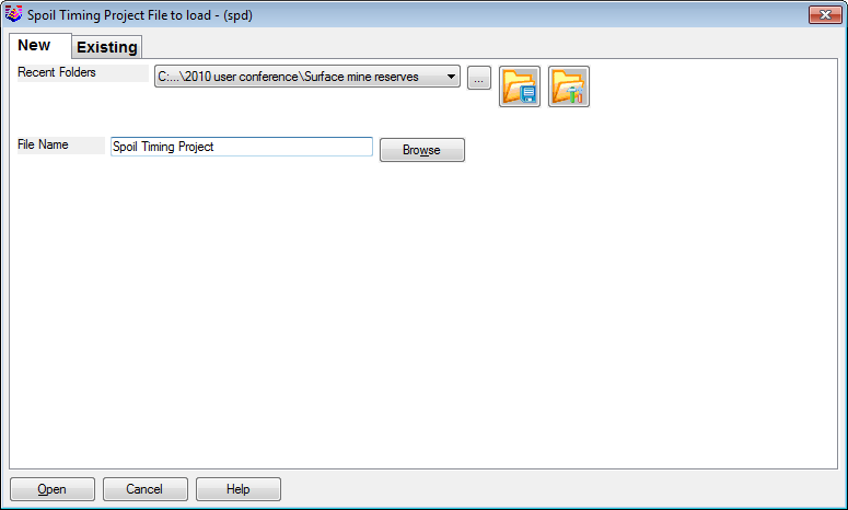
The first window is to select a new Spoil Timing Project file, or
load an existing one (*.SPD file).
 Once the SPD file is named, then the Fleets and
production are defined in the next window, if there aren't any in
the file already. The green + and X buttons are for adding and
deleting the rows. Give each fleet a name and a production per
hour, and hours per day worked on average. If a fleet is already
saved, it can be loaded with the Load button.
Once the SPD file is named, then the Fleets and
production are defined in the next window, if there aren't any in
the file already. The green + and X buttons are for adding and
deleting the rows. Give each fleet a name and a production per
hour, and hours per day worked on average. If a fleet is already
saved, it can be loaded with the Load button. 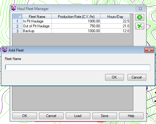 The
next step is to load the Spoil Source file (*.SPO) that was created
with either Surface Mine Reserves or Surface Equipment Timing.
The
next step is to load the Spoil Source file (*.SPO) that was created
with either Surface Mine Reserves or Surface Equipment Timing.
 The Spoil Source editing window will appear
next. This gives the opportunity to review the source data and make
any final edits before scheduling. The data in the image below came
straight out of the Surface Equipment Timing command.
The Spoil Source editing window will appear
next. This gives the opportunity to review the source data and make
any final edits before scheduling. The data in the image below came
straight out of the Surface Equipment Timing command. 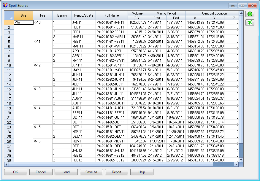 The
next screen will be the Spoil Timing Project manager. This shows a
tree structure of the project which is comprised of 3 main areas,
including the Haul Fleets, Spoil Sources and Spoil Destinations.
The
next screen will be the Spoil Timing Project manager. This shows a
tree structure of the project which is comprised of 3 main areas,
including the Haul Fleets, Spoil Sources and Spoil Destinations.
 After the Spoil Timing Project screen, where
all the items can be viewed and edited, clicking OK brings up the
Spoil Placement Timing window. This is where all of the assigning
and reporting of the schedule is set.
After the Spoil Timing Project screen, where
all the items can be viewed and edited, clicking OK brings up the
Spoil Placement Timing window. This is where all of the assigning
and reporting of the schedule is set.  This
is the main dialog for sequencing the spoil timing. It is divided
into 4 main areas, and they are described with the matching numbers
labeled on the image for clarity.
This
is the main dialog for sequencing the spoil timing. It is divided
into 4 main areas, and they are described with the matching numbers
labeled on the image for clarity.
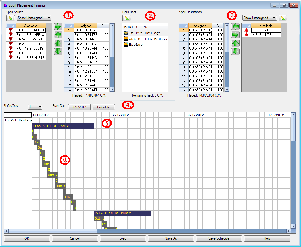 1. Spoil
Source section shows a list of available spoil sources from
the Spoil Source file that was used. They can be edited with the
button, and sorted up or down. The procedure is to move them from
left to right, in order to be filled by the mining.
1. Spoil
Source section shows a list of available spoil sources from
the Spoil Source file that was used. They can be edited with the
button, and sorted up or down. The procedure is to move them from
left to right, in order to be filled by the mining.
- 2. Haul Fleet: This
section shows the list of haul fleet units that are defined. Edits
can be made here. To set one current, just pick it and keep it
highlighted while timing spoil.
- 3. Spoil Destination
section is the method to define where the spoil cuts are going. In
this example, there are both in pit and out of pit spoil locations.
Multiple benches will be displayed with B1, B2, etc.
- 4. Calculate is used to
run the timing and get the reports once the spoil sources have been
assigned to a destination. Enter in a start date if it is changed.
The Shifts/Day displays how many divisions are displayed in the
white window below. The gray grid lines are the shifts per month.
If only 1 shift per day is selected, then each grid line is a full
day.
- 5. Each period is divided by the red, vertical lines. This
example shows months.
- 6. The dark blue gantt chart bars are the spoil sources. The
gray bars are the spoil destination perimeters. Each spoil source
has to go somewhere, once that source is used up, then the
destinations go to the next source.
Once selecting the Calculate button, the next window determines the
type and options for reporting. If any of the report types are set
to just periods, then the window will appear like this. 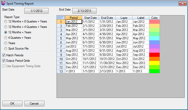 If
the Spoil Source File is selected, then the periods set there,
created from Surface Equipment Timing, will set the period
intervals. This also activates the Use Equipment Timing Grids,
which will use the GSQ grid sequence file, and merge that with the
spoil surfaces per period.
If
the Spoil Source File is selected, then the periods set there,
created from Surface Equipment Timing, will set the period
intervals. This also activates the Use Equipment Timing Grids,
which will use the GSQ grid sequence file, and merge that with the
spoil surfaces per period. 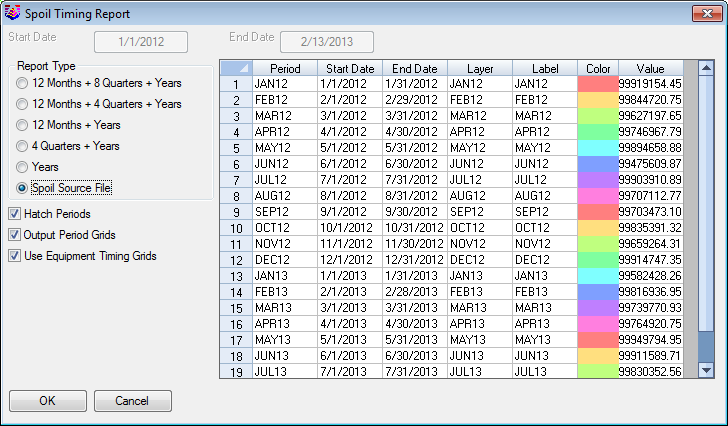 To
select the output grids for the 3D spoil results, the surface
topography, final ground surface grid is set here. Also, the top of
each bench grid file is set here, for multibench spoil. These grids
can be made with Grid File Utilities to set the designs by area or
inclusions. For example, the top of Bench 1 could be a combination
of the post mining topography for in the pit spoils, and a fill
design elsewhere, for out of pit spoiling and dumping.
To
select the output grids for the 3D spoil results, the surface
topography, final ground surface grid is set here. Also, the top of
each bench grid file is set here, for multibench spoil. These grids
can be made with Grid File Utilities to set the designs by area or
inclusions. For example, the top of Bench 1 could be a combination
of the post mining topography for in the pit spoils, and a fill
design elsewhere, for out of pit spoiling and dumping. 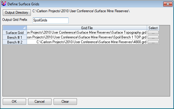 The
program will now prompt for the existing GSQ Grid Sequence file to
use. This file contains the advance of just the pits in the mining
sequence. It will now use this file, matching up the periods, and
add in the back fill spoiling. This will represent the full mining
progression, showing the advance of the pits, and the following of
the spoil and dumps.
The
program will now prompt for the existing GSQ Grid Sequence file to
use. This file contains the advance of just the pits in the mining
sequence. It will now use this file, matching up the periods, and
add in the back fill spoiling. This will represent the full mining
progression, showing the advance of the pits, and the following of
the spoil and dumps. 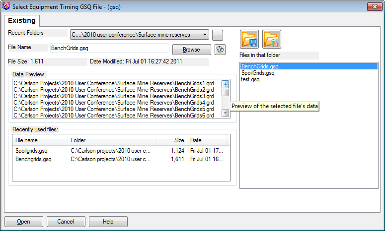 The plan view map is hatched with the
color period blocks to illustrate where each spoil is placed in
each period.
The plan view map is hatched with the
color period blocks to illustrate where each spoil is placed in
each period.  This creates a new GSQ file, with the name
defined above in the Define Surface Grids window. It uses the name
define here by default, SpoilGrids. Viewing this file with the View
3D Surface History will show the mining progression with the spoil
fills.
This creates a new GSQ file, with the name
defined above in the Define Surface Grids window. It uses the name
define here by default, SpoilGrids. Viewing this file with the View
3D Surface History will show the mining progression with the spoil
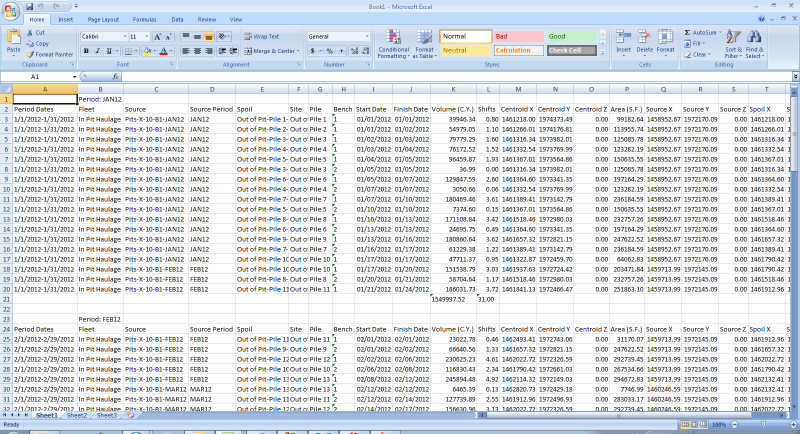
fills. 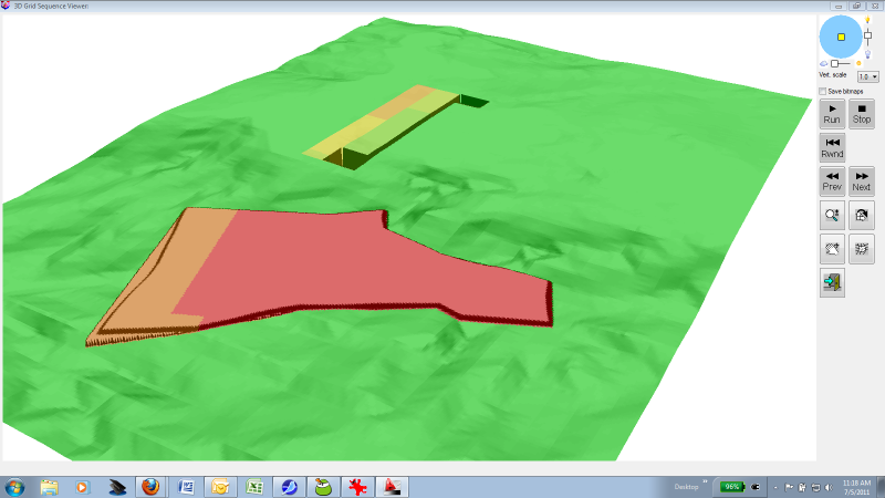 Using the Report Formatter can export the
report directly into Excel. An example Excel dump is shown here.
Using the Report Formatter can export the
report directly into Excel. An example Excel dump is shown here.
 Keyboard Command: timespoil
Prerequisite: SPO file from Surface Mine Reserves or Surface
Equipment Timing, spoil polylines with direction, and haulage
fleet.
Pulldown Menu Location: Spoil in Surface Mine Module