
The following is an introductory tutorial for Carlson Point Clouds. If you wish to follow along with the tutorial and use the same Scan files, you can download them from the Carlson website at http://update.carlsonsw.com/tutorials/pointcloud/data.zip
These files aren't required, however, and you can follow along with any set of scans that have proper target points and control points.
Work done in Carlson's Point Cloud module is done on a per-project basis. To create a new project, you must first have a CAD drawing open in AutoCAD or IntelliCAD. To load the Point Cloud menu structure, click on the Lightning Bolt icon, or load it through the menus by going to Settings ⇒ Carlson Menus ⇒ Point Clouds.
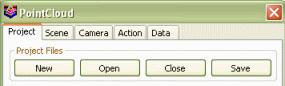
This will display the menu structure for Point Clouds. Now select Point Clouds ⇒ Project Manager. Then select New for a New project. Select the file path where you want it stored, enter in a filename and then click on Save.
Your initial project should look like the following image. In the tree structure you will see your Project with various defaults.
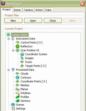
First, let's change some general project settings. This will allow the units, the look and the feel to be correct for your environment. This can be done either by double-clicking on the Settings item in the tree, or by a right-clicking the Settings item and selecting View from the menu. In the Units and Ranges section, you may change the project's units between Meters or Feet, which is the default. For this exercise, select Meters.
The Naming Conventions section allows you to change the settings for the naming of various fields. Look over the defaults, and if you wish to change something to your liking, please do so.
Finally, take a look at the Viewer section and make any changes to the defaults if you desire.
Once this is done, click on the green check mark button to accept the Project settings. Typically, to accept the results of or continue with a function you should click the green check mark button; if you want to cancel a process click the red X.
The tutorial scan set that is supplied for this exercise will consist of three different scanner setups, each having obtained a scan in their own scanner coordinate system. Included with these scans are targets scans for each scan and the control coordinates for the site. This will allow us to complete a full registration of the three point clouds, and merge them into one entity for further manipulation.
Let's begin by adding two more scan position trees.
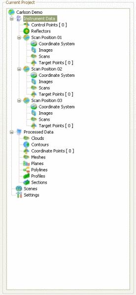
Right click on Instrument Data ⇒ Add ⇒ New Position. Do this one more time, to have a final count of three Scan Positions, as per the diagram below.
We will now proceed with adding the information to the scans.
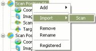
Right click on Scan Position 01 ⇒ Import ⇒ Scan.
It will now displayed another dialog box asking you for the text file that has the necessary scan data in it in symbol delimited format, consisting of X, Y, Z, Intensity and R, G, B values.
Navigate to where the scans you wish to use and select the scan file. If you're using those from the Carlson website, select the following file: Color_ScanPos01 - Pa01.txt
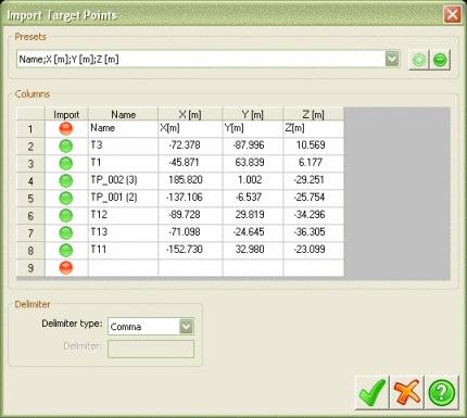
You will now see an Import Scan dialog box.
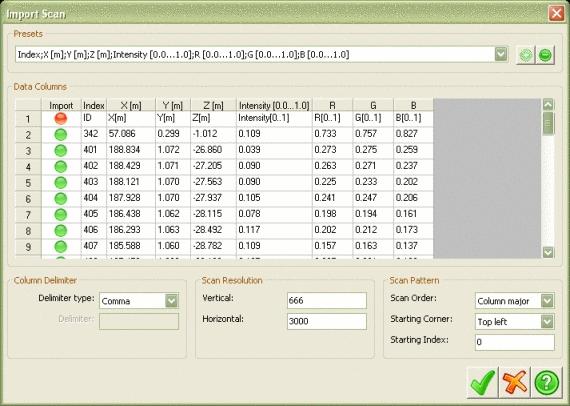
Click on the green button under the heading Import, and it will change to red. This means it will not import that line of text. Typically, the first line in a text scan file will be a list of data types and should not be imported.
Now, we need to assign each of the fields with their respective information. This is done by left-clicking on the column headers and selecting the data type for that column. Click the column header above X[m], which should be in the first row of data, and select X[m] from the drop down menu. Continue this process for each column of data until all of the columns have the proper headers.
To store this header arrangement for future use, click on the green plus sign button and it will assign a preset for you. This column header preset can now be used every time you import scan files with the same data ordering.
Now you will need to enter in the scan resolution values as well as information about how the scan data is oriented. If you're using the data set from the Carlson website, please refer to the supplied Dimensions.txt file for this information on the three scans.
After clicking the green checkmark you should see the scan import progress dialog.

Continue to import the other two scans to their respective scan positions, this time you can utilize the preset made from the first one by selecting it from the presets drop down box. Once the scans have been imported, each of your scan position trees under the project should have the following structure:
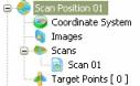
Now let's import the scanned targets for each of the scans, and the control for the registration process. This procedure is similar to importing the scan. The only difference is that you now right-click on Target Points [0] for each scan and select Import.

You will have various options, if required, for importing the points. For the tutorial dataset, make sure the Rename all items checkbox remains unchecked and the Ignore Duplicates radio button is selected. Once these are done click on the green check mark to accept your choice. You will now see that the zero value has increased to 7.

Continue to import the Target points until each of the scan positions have their target scans imported, and then do the same with the Control Points, which is at the top of the tree.

Once all of this has been done, click on Save to perform a save of all the data that has been imported.
This is done by going into the scanned target data and applying a registration to the control.
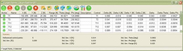
Double left click on the Target Points in the scan tree, or right-click ⇒ Edit and it will display a window to the above diagram. The information displayed in the spreadsheet can be modified by clicking the Settings icon and modifying them to your liking.
Once this is done, click on the Register Scan Position icon and a popup will appear as shown below.

Set the method to Minimize point position error. You may need to up the value of the Maximum Error to allow for a larger search radius until all of the points have been matched.
Look at the residuals and make sure that are to your satisfaction. Each scan will differ. Once this is done, it will inform you that the registration has been successful. Continue registering target points in other scans until all scans are registered.
Now each of the Point Clouds has a different co-ordinate systems assigned to them.
Now we will create a view and add all the scans to the same view for further manipulation.
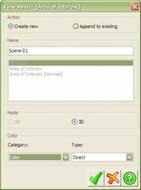
Select Scan Position 01 - Scan 01 by either a double left-click or right click ⇒ View and it will open a dialog box as seen below.
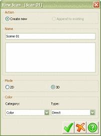
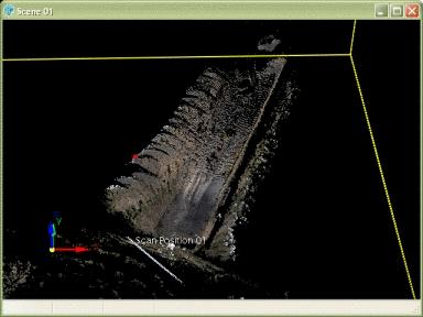
Select the Create new option, and leave the default name for the Scene. Remember the scene name for later, as you're going to add the other scans to it. Set the display mode to 3D and in the color panel choose Color for the category and Direct for the type. After clicking the green check mark a new window should pop up after the scan has loaded that shows a scene similar to the one below.
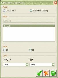
After creating the initial scene, go back to the project manager and right click Scan Position 02 - Scan 01 and select View. This time we will choose Append to existing and select the Scene created from the last scan. Make sure the coloring options are the same as the other and that the Mode is set to 3D and click the green check mark.
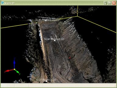
Your scene window should update to reflect your changes. Repeat this process again for Scan Position 03 - Scan 01 and add it to the same scene. Your final scene should look something like the one below.
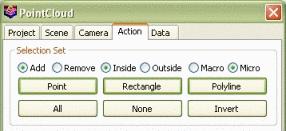
The scanner has picked up some points outside our area of interest. To eliminate them from the data set, click on the Action tab and use the Polyline Selection tool to select the desired data points. Make sure the Micro selection mode is on. Macro mode means that if any part of a dataset is selected, that entire dataset is selected, which is not the selection behavior we want here.

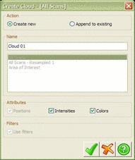
Make a new Cloud from the selected points by clicking Cloud in the create panel of the Action tab. This will launch the Create Cloud dialog. Click the green check mark to create a new point cloud containing just the selected points. You can locate the new cloud under Project ⇒ Processed Data ⇒ Clouds.

The new point cloud contains data from three different scan positions. Inevitably, some of the data points are duplicated in the areas where scans overlap. You can now resample your cloud to eliminate unwanted data points.
To do so, right click on the cloud in the Project tab, and select the Resample option. This will bring up the Resample Cloud dialog.
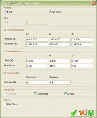
The Oc-Tree resampling method typically provides the best results. Leave the Oc-Tree dimensions unchanged, and specify Oc-Tree Resolution and Node settings as shown. Click the green check mark to create your new, resampled point cloud. This process may take a few minutes. After it is complete, you will have a new resampled cloud under Project ⇒ Processed Data ⇒ Clouds.
Now that you have isolated and resampled your area of interest, you can make a triangulated mesh surface from your data points.
The simplest way to do so is to right click your resampled point cloud and select Create ⇒ Mesh. This will launch the Create Mesh dialog.

Change the maximum edge length setting to 50 meters and maximum incident angle to 90°; this will prevent valid triangular faces from being eliminated during the triangulation process. Click the green check mark to create your mesh. This process may take a few minutes. After it is complete, you will have a new mesh under Project ⇒ Processed Data ⇒ Meshes.
You can export a mesh to a Carlson 2007 TIN file by right-clicking on it, and selecting Export.
The next task is to automatically draw in breaklines for top and bottom of bank of the data set. To do so, right click your mesh and select View. This will launch the View Mesh dialog.
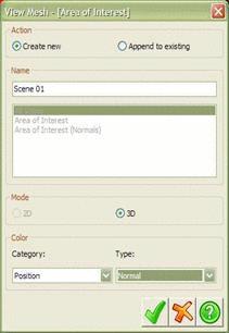
Select Position for Color Category, Normal for Color Type and click the green check mark to view your mesh.
Each vertex in your mesh is colored according to the direction of the normal vector. Think of it as the "up" direction.
The axis icon gives you a good idea of how the colors are assigned. Its x-axis is colored red, y-axis is colored green and z-axis is colored blue.
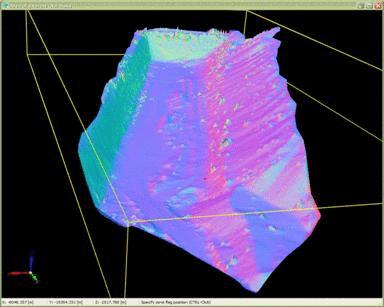
Vertices that "face" the x-axis have a higher saturation of red, vertices that "face" the y-axis have a higher saturation of green and vertices that "face" the z-axis have a higher saturation of blue.
Access the Action tab and select all the vertices in your data set. The simplest way to do so is to click the All button with the Add radio button selected.
Initiate the breakline extraction process by clicking Extract Breaklines in the Action tab. This will display the breakline extraction options panel.

The next task is to set up your Direction - Color zones. To create a zone, ctrl-click on a data point inside the viewer. To delete one or more zones, highlight them in the spreadsheet, and click the Delete button.
Think of zones as groups of points which all face a similar direction. In this particular example, there are two such groups: points in the flat area on the bottom of the trench (low slope) and points on the walls of the trench (high slope). Ctrl-click on one sample point in each zone.
Click the Show button to preview your zones. At this stage, for each point in your selection set, the program figures out which of the sample points it is most similar to, in terms of orientation or color, and shades it accordingly.
The breaklines will be extracted at the boundaries between adjacent zones.

Active Directions - Color toggles help you fine tune zone processing. For example, two data points may have similar facing along the x-axis but vastly different facing along the z-axis. This would be indicated by similar red values but different blue values.
You can examine the value of any data point under your cursor in the Data tab. This helps with setting up your zones.

Also, you can use Zone smoothing settings to get rid of some of the unwanted noise inside the zones and along the zone boundaries.
To extract the breaklines, you need to specify the maximum distance between adjacent breakline, as well as the smoothing and simplification settings.
Once you are happy with the zones and the preview, click Extract to extract the breaklines and view your results.
Your breaklines will appear under Project tab ⇒ Processed Data ⇒ Polylines. You can delete unwanted polylines by right-clicking on them, and selecting Remove.

In this particular example, the automatic breakline extraction is not sensitive enough to detect outlines of roads at the bottom of the trench. These road features can be surveyed in manually.
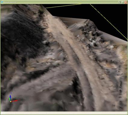
To do so, close the current viewer, then right click your mesh and select View. This will launch the View Mesh dialog.
Select Color for Color Category, Direct for Color Type and click the green check mark to view your mesh.
Access the Action tab and click Point in the Create panel. This will display virtual survey options.
First, select Coordinate Points from the choices in the Active List box. This means that each point you create is a common coordinate point (not a control or target point used for registering scans).

Next, specify a suitable point name (sometimes called point number) and a description for the next point you are going to create. You can use the Pick button to access the contents of your current field-to-finish codebook file.
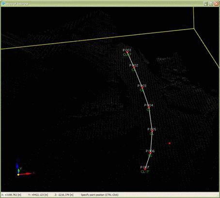
Ctrl-click in the viewer to create new coordinate points.
Field-to-finish linework will be generated automatically according to your field-to-finish codebook. You may also use the Linework portion of the dialog to append special codes to your coordinate points.
You can view and edit coordinate points that you have already created by right clicking on Coordinate Points and selecting Edit in the Project tab.
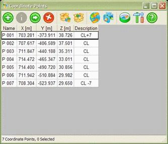
You can export your coordinate points to a CRD file by right clicking on Coordinate Points and selecting Export in the project tab. (CRD is one of several available formats.)
This completes this Point Cloud Step-by-Step tutorial.