Production By Block Model

The Production By Block Model is intended to organize grids or triangulation files created by the Carlson Software Civil Design or Mining modules into mineable blocks. The software analyzes each block to report the amounts and qualities of each seam contained in the block. During layout, the analyzed blocks may be subdivided along elevations, or along strata intersections. Only the top-most block in a series of stacked blocks is “active” to the software. Once a block is mined, the next layer of blocks becomes available for selection. Once the model is built, the model files may be transferred to any computer, with or without Carlson, to allow mine personnel to query, build mine plans, and/or mark blocks as mined. The following diagram illustrates the concept where the example blocks are shown in bold.

The block size may be determined to represent an economically viable mining volume, a series of bench elevations or any combination of layout. Blocks may be any size and shape with a single set of requirements:

All blocks stack on top of similarly shaped blocks,
Blocks are arranged in a series of constant thickness.

1. Setting Up The Pick and Choose Model

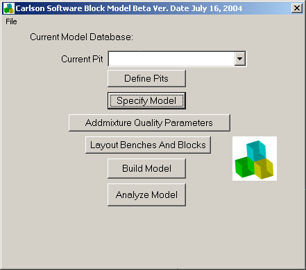
The process for analyzing the Block Model is as follows:

Define the Pits (Separate Mining Areas)
Define the Carlson grid or TIN files that describe the subsurface for each pit
Define Admixtures (future enhancement)
Layout Blocks for each pit
Build The Model for each pit
Analyze the model

The menu structure of the software is organized in the same order:

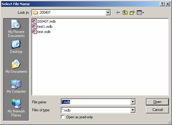
The first step is to give the model a name. That can be accomplished under the File pulldown menu, Set option. Alternatively, the software will ask for the same information if any other button is pressed before setting the model file. The screen will appear as:

Enter the name and location of the model. If you enter a file that does not exist, the software will ask if you want to create a new one.

2. Defining Pits

Pits are simply names of separate mining areas. Each area has it own set of grid files, even the files are the same throughout the project. All projects must have at least one pit. New models include this pit and assign its name as ‘Default’. Press the “Define Pits” button on the main screen to rename, or add pits. The screen will appear as:

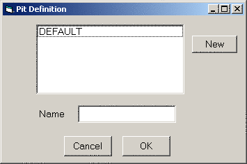
Click on a Pit Name in the list. The name will appear in the bottom entry box. It may be edited there. The pit named DEFAULT may not be renamed unless more than one pit exists.

Press the New button to add a name. A box will appear where the name can be entered for the new pit. When pits are renamed in the bottom box, the change is not recorded until you click on another name in the list. The Cancel button will discard all changes made while on the screen.

3. Specify Model

Set the model file, and the pit on the main screen shown here:

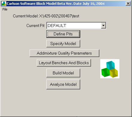
This shows where the model is set to X:\425-002\200407\test, and the pit is set to DEFAULT. Press the Specify Model to obtain a page similar to:

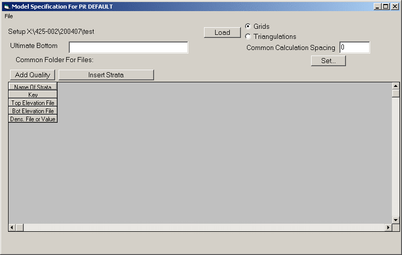
The mining model entry is made in the grid or spreadsheet on the dialog. Mining materials (strata) are defined along the top of the spreadsheet, and attributes (qualities) are listed along the left edge. Every material in the block has the opportunity to relate to every quality. Items that do not apply, are simply left blank in the grid.

Grid or triangulation files may be entered as the defining limits and the qualities of the materials in the blocks. The files are NOT required to be of equal spans, or spacing in grids, and do NOT need to be of similar shape in triangulations. They should, however, cover the entire area of the block model. Blocks falling outside the file limits of a particular area will have that particular volume or quality set to nothing (no data.)

The first pit in the list (DEFAULT or to whatever it has been renamed), defines the material(s) and attached quality(s) associated with each material. All materials (strata) and qualities used in each pit must be defined in the first pit, even if they do not exist. Calculations are made on a regular spacing in the limit of the blocks. This calculation spacing is defined by the user in the box ‘Common Calculation Spacing.’ This box must be filled in on the first pit, before the entry page is saved to the model or the software warns that it is blank.

4. Manual Entry:

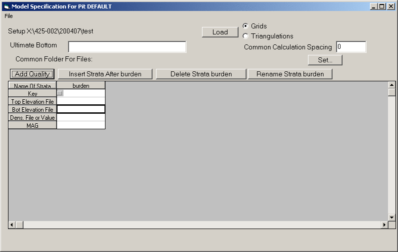
Adding materials: Insert a material (strata) by pressing the Insert Strata button. Enter a name in the box and press enter.
Adding qualities: Insert a quality (attribute) by pressing the Add Quality button. Enter a name in the box and press enter.

The example entered here was ‘burden’ as a strata, and ‘MAG’ as a quality:

5. Entering File Names In The Spreadsheet:

Move the cursor to an appropriate cell in the spreadsheet and double-click the cell with the mouse. Select the file and press OK. The file name will appear in the box. Materials are defined as top and bottom elevations or a series of thickness files. To establish elevations, the first (top most in the model, left most column in the spreadsheet) material is required to have a structure, or elevation file in the box labeled Top Elevation File. The remainder of materials require only a bottom structure or thickness file. All materials must be defined the same way, bottom elevations, or thickness. To toggle between elevations and thickness files, double-click the left-most spreadsheet cell, fourth row down. The label will change “Bot Elevation File” and “Thickness”
Once the spreadsheet is complete, select the File pulldown, Save and Exit option. Be careful, as CLOSING THE SCREEN WITH THE X IN THE UPPER RIGHT CORNER OF THE WINDOW, IS EQUIVALENT TO CANCELING THE ENTRY.

Options:

Using Scalar Numbers: If a grid or triangulation file does not exist, and an assume number is to be used, type the number in place of a file. Note: If a file exists with the same name as the number, the file will be used. For example entering a scalar of 123, when a file 123.GRD exists, will cause the program to use the file.

Grids or Triangulations: Clicking the option Grids, or Triangulations will limit the list of possible files when selecting a file. Also, if the file selected is a grid file (.GRD extension) and the Grids option is selected, the extension of the file is not shown in the spreadsheet cell. The same holds true for triangulation files.

Ultimate Bottom: If a Grid or Triangulation file exists that defined the bottom of mining, enter the file in the Ultimate Bottom box (double-click for a file list.) All blocks or portions of blocks falling below this bottom will be trimmed to that file, or discarded completely as needed.

Common Folder For Files: Each Pit may refer to a different folder on the hard disk. This folder can be set with the Set button to the right of the ‘Common Folder For Files:’ label. This will be the default folder to search in file selection. If selected files are in that folder, the folder path will be removed in the spreadsheet display. If a file is selected outside that path, then the full name, including the path will appear. Changing the common folder will change all files to reference that path, if the files exist.

Key:Volumes and Weights are split into two categories, Key and Non-Key. Totals for each material are given during block mining, as well as total weighted values for Key and Non-Key.

Density: All materials are reported as volumes and converted to weights by either a density grid, or scalar. The weights are then used to report weighted averages of the qualities. A zero is allowed, but discouraged to properly weight averages. If no values are available, use the same scalar for each material. The number 1 is acceptable for such a situation.
Using A Carlson Geologic Model File:A Carlson Geologic Model file may be used to fill in the spreadsheet. The behavior of the option differs depending on the status. If no materials or qualities have been defined ( a new model), all material (strata) in the Geologic Model file will be added. The user may pick all or some of the attribute (qualities) in the file to use in the block model. If materials and/or qualities have been defined ( a new model), all materials (strata) and attributes (qualities) in the Geologic Model file that match the names in the block model will be examined by the software. Spreadsheet cells that are blank and match the Geologic Model file, will be filled in.
AutoFill Right: After at least one material has been added to the model, the AutoFill Right button will appear. After filling in file names for the first strata, the AutoFill Right button may be useful. If all files for each strata are named similarly, the software can make some intelligent selections of files. For example see the following example:

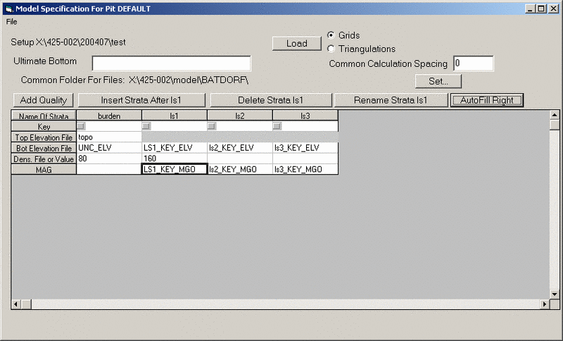
The model has three strata, ls1, ls2, and ls3. The file name values are entered for ls1, but are blank for ls2 and ls3. The common folder path is set to X:\425-002\model\BATDORF. By placing the cursor in any cell under the ls1 heading, and pressing the AutoFill Right button, the software looks for files that have the ‘ls2’ where the ‘ls1’ occurs in the previous files. It repeats the process for each blank cell, under each named strata. Because the files existed in folder X:\425-002\model\BATDORF for this example, the screen now appears as shown below. This example shows the benefit of using consistent naming practices in Carlson.

6. Copying Files From Other Pits

After the model is set up in the first pit, the basics are complete. However, additional pits still need to have reference to appropriate files for those pits. If model files are being entered for a pit other than the first pit, another option is available under the File pulldown menu. It will appear as “Copy From Pit <NAME>” where <NAME> is the name of the first pit in your project. If this button is picked, an exact duplicate is made of the default (first) pit.

If the names of the files are the same as the first pit, but the folder they are in is different, simply copy the first pit files, and change the Common File Folder. If the files exist, they will redisplay. Files that do not exist are shown in red. You may also copy files into the first pit from another block model file if the current model file is newly created. Select the option under the File pulldown, select the database, and the files are filled in.

7. Laying Out Blocks

Block outlines are generally simple a series of boundary lines stacked one on top of the other throughout the reserve. Generally the block height represents a single bench elevation used in the mining. For example, look at the example below of a pit with a ramp, created with the Carlson Process Fill/Cut command, and rendered with the 3D Viewer.

If we look at a plan view of the pit, contoured at the bench elevations, we would see something like the following:

The contour lines at each bench elevation become the limit of blocks we are going to create. Blocks outside those lines are not accessible, and do not require storage in the block model. The software allows each level of stacked blocks to have its own limiting boundary. In the case of a single bench mine, a single boundary line is all that is required.

8. Block Bench Entry:

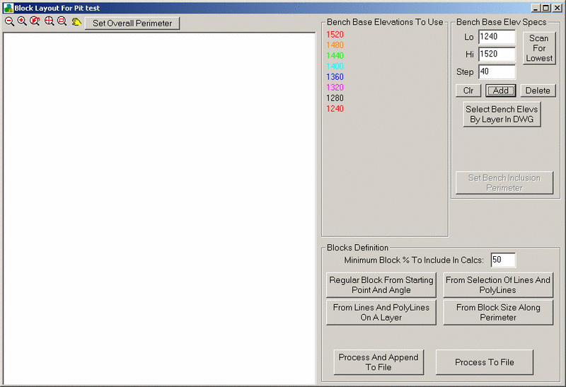
Set the appropriate pit on the main menu, and press the Layout Benches And Blocks Button. The screen will appear similar to:

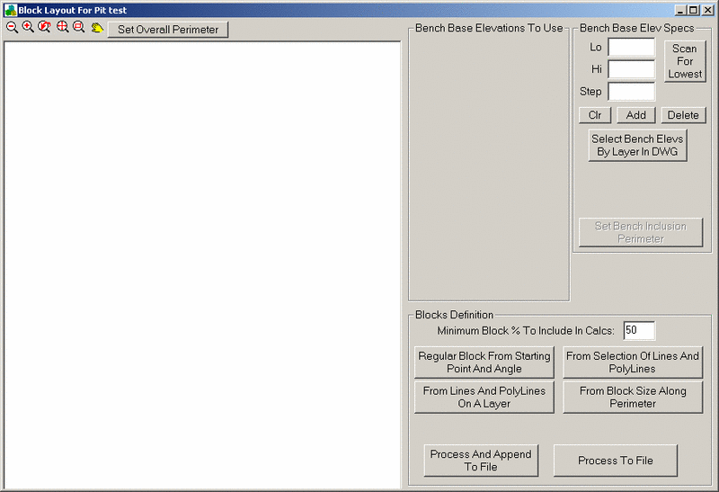
The buttons in the top left corner control the zoom level and view by Zooming Out, In, Previous, Extents, Window, and Pan, respectively.

Block definition is divided into two portions. The first option is Definition of Block Base Elevations. The second option is the Definition of Block Boundaries.

Block Elevation boundaries (Benches) can be accomplished by two methods:

Manual Entry Block Base Elevations

Step 1:
Enter low, high, and spacing (step) values of benches in the upper right boxes. Pressing the Add button places the values in the frame labeled Bench Base Elevations To Use. For example, suppose the bottom of the pits were at elevation 1240 with bench elevations of 40 units extending upwards to the highest bench of 1520. With those values in the appropriate boxes, pressing the Add button results in:

The list of elevations now shows in the Bench Base Elevations To Use frame, sorted highest to lowest. Each has a color attached to help differentiate the boundaries. To enter a single elevation into the list, put the single elevation value in the Hi, and Lo box, with a Step =1, and press the Add button. As many as required may be entered. The values do NOT need to be equally spaced.

Step 2:
Once all the elevations are set for the benches, each must be assigned a limiting boundary line. Click the mouse on one of the elevations. The elevation will turn bold. In the example below, elevation 1520 was selected:

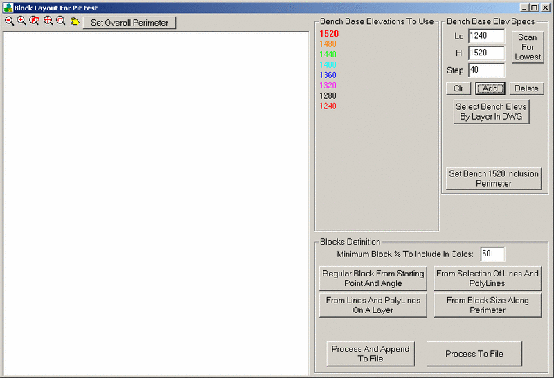
The bottom button in the Bench Base Elevations frame now says “Set 1520 Inclusion Perimeter” Press that button to select the boundary line in AutoCAD. Once selected, the screen will reappear. In this case the outer-most boundary line from the contours shown earlier was selected and the screen returns:

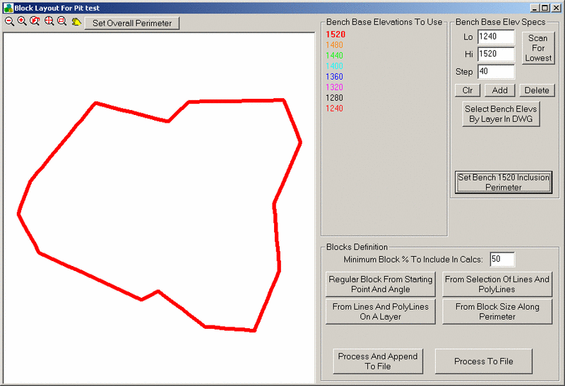
Repeat Step 2 for Each boundary line until the screen appears similar to:

Note that the selected elevation in the list highlights the appropriate boundary line on the drawing.

Automatic Entry of Block Base Elevations
If the limiting lines for each bench are already drawn on a single layer in AutoCAD, and are 3D Polylines, or 2D Polylines with elevations (as drawn by the Process Fill/Cut command, or Contouring routines in Carlson), the software can use them automatically. The button labeled Select Bench Elevs By Layer In DWG accomplishes this task. Pressing that button switches to the AutoCAD drawing and prompts the user to select a single entity. Note: All entities on that AutoCAD layer are examined so the boundary lines should reside on a layer to themselves (no other polylines on the layer). When the selection is made, the following prompt will occur:

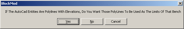
Selecting Yes causes all elevations to be added to the list automatically, and the polylines attached. Choosing No causes only the elevations to be added to the list (no boundary lines.) In this case, Yes was selected. Press the Zoom Extents button to see the boundaries.

Definition of Block Boundaries
Regular Blocks
Block boundaries are defined in with the options in the lower right box on the page. The simplest option is the button “Regular Block From Starting Point And Angle.” The option creates rectangular shaped block boundaries based on a selected orientation. When this option is selected, the screen switches to AutoCAD.

The program prompts: Select One Corner Of A Block, - Inside AutoCAD, select the corner.
The next prompt is: Select Angle Along Block Face - Use AutoCAD to select the orientation.

The pit layout screen reappears prompting for the length and width of the block faces. The software then draws the blocks on the screen that could possibly be present. The following screen is an example where square blocks were selected:

As the screen above indicates, some of the blocks are outside the perimeter, some are inside, and some are partially in, partially out. This shows the need for some method to decide whether the block is included in the model or not.

The box labeled “Minimum Block % To Include In Calcs” allows the user to enter a threshold for using the block or not. A value of 100 would include only blocks completely inside the perimeter(s) of the elevation benches while a value of 1 would include any block inside or touching the perimeters. Regardless of the value entered, the percentage of each block contained inside the perimeter is stored along with the block model. When the blocks are mined, the percentage is applied to the recoverable volumes and weight.

Arbitrary Blocks
The following is the perimeter of the example Inside Of AutoCAD. It has a series of interior lines drawn at pit boundaries (blue ends indicate the grips from selection in the drawing):

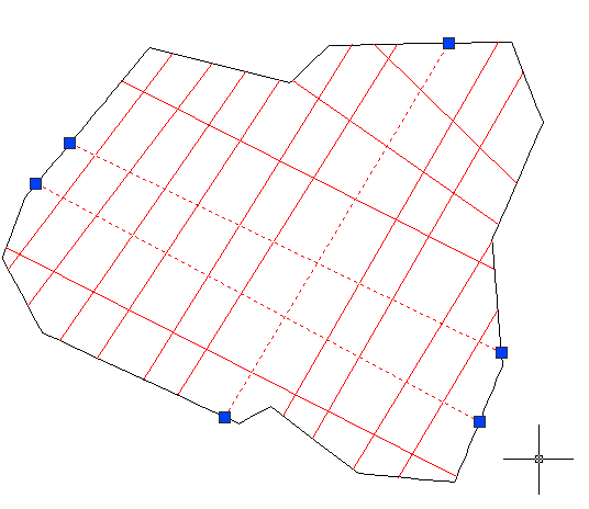
The arbitrary block algorithm uses a polygon processor logic to create the polygon block boundaries from primitive lines and polylines.

Option1: From Selection Of Lines And Polylines - This option allows a selection set manually made in AutoCAD.
Option2: From Selection Of Lines And Polylines On A Layer - This option allows a selection set made by selecting a single entity in AutoCAD. The software then gathers all entities on that layer to use for the selection set.

Regardless of the option, the software starts with the prompt:

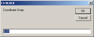
Coordinate snap is a method to force the selected line segments to intersect, or trim as needed automatically. It helps clean up loosely drawn geometry to create perfectly matched polygon edges. The following demonstrates the affects of coordinate snap:

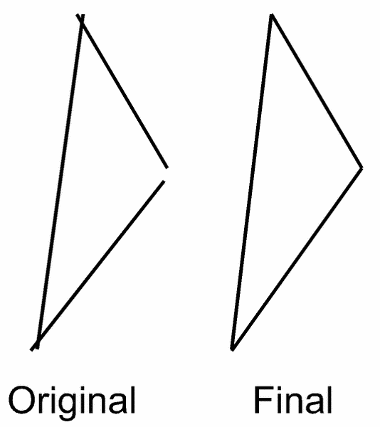
Any small number is acceptable, depending on the integrity of the primitives selected. If gaps and overhangs occur in the drawing larger than the entered snap, the user is warned. Red circles are also drawn in the AutoCAD drawing where the errors exist to aid in correcting the primitives. Assuming Option 1 is selected, and the lines shown in the last diagram are selected in AutoCAD, the screen will return as:

Depending on the complexity of the geometry, a small amount of time may pass as the software build the polygons.

Saving The Block Boundaries And Elevation Limits:
Process To File, and Process And Append To File accomplish the same task, building the block model. Process To File erases any existing definitions of blocks for this pit, rewriting them completely. The Process and Append leaves existing blocks, adding the new ones described in the page. A progress bar appears on the screen to indicate progress. The process run time is completely dependent on the total number of block, total number of elevations (benches), and the complexity of the geometry. This process of building blocks is required for each pit separately.

9. Building The Model

This section is fully automatic after setting the active pit and pressing the Build Model on the main screen. Optionally, you may use the File pulldown menu >Build All Pit Models. This option runs the model for each pit, one at a time. The routine interpolates each structure and quality file in the model at the common resolution, applies them to each block, and summarizes the block in the model. It is the most computer intensive section of the block model program.

All summaries are kept in the model file itself. For example, if the model is name Test, the summaries are all in the disk file Test.mdb The software also creates a series of model files for each pit. If we had three pits defined, three additional files would be made: Test1.mdl, Test2.mdl, and Test3.mdl. These files can be quite large depending on the detail of the user selections. However, they are quite useful in analyzing the model (next section.) The software uses the files to instantly re-analyze blocks, should you choose to split a block on elevation boundaries.

Updating A Model With New Information
As is generally the case, continuing mining activities yield more and more information. Should additional holes be drilled, or pit samples added to the Carlson model, the user may choose to rebuild the grid or TIN files used by the model. If that is the case, and the changes warrant updating the blocks, building the model is a simple as pressing the Build Model button.

However, this is true only if the model names are unchanged, and the block layouts have not changed. Those changes require re-entry of the applicable data before building the model.

10. Analysis

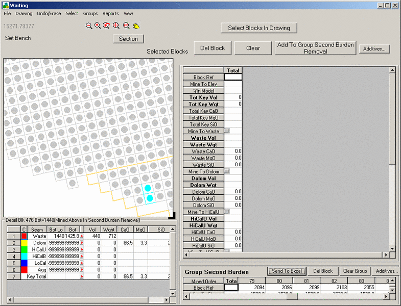
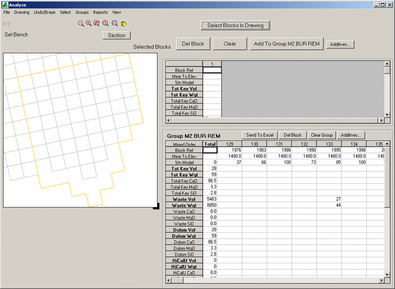
After the model is built, press the Analyze Model button on the main page. The screen appears similar to this:

Using The Screen

Placing the mouse on the small corner at the lower of the drawing on the left, pressing the left mouse button, and holding it down, sizes the drawing window.
Placing the mouse between the two spreadsheets shown by blue line above (not on the actual screen), pressing the left mouse button, and holding it down and moving the mouse up-down, sizes the spreadsheet windows heights.
Placing the mouse between at the left of the top spreadsheet shown by blue green above (not on the actual screen), pressing the left mouse button, and holding it down and moving the mouse left-right, sizes the spreadsheet windows widths.
The drawing may overlap the spreadsheet or vice versa. Clicking the mouse in either one cause that section to be on top.
The spreadsheets have control bars to slide up-down or right-left in the data.
Spreadsheet column widths are adjusted by holding down the mouse on the line between columns in the header section of the sheet and dragging. All columns in both sheets reflect the new column width.

Basic Concepts:

Blocks are selected in the drawing area.
Blocks are selected from the top down.
Selected blocks go into the temporary work area for viewing of data.
Once satisfied with the temporary data, the data is moved into the current group.
Groups are simply user defined mining areas of multiple blocks.

Selecting Blocks (Blocks are selected in multiple ways):

Place the mouse inside the block and left click.
Hold down the shift key, and the mouse left button. Move the mouse over block. Blocks are selected as the mouse touches them.
Use the Select Pulldown > Fence. Draw a polyline on the drawing by subsequent clicks of the mouse. Press the End Select button after the last point. All blocks touching the polyline are selected.
Use the Select Pulldown > Window Poly. Draw a polyline on the drawing by subsequent clicks of the mouse. Press the End Select button after the last point. The polyline is closed automatically. All blocks inside the polygon are selected.
Use the Select Pulldown > Crossing Poly. Draw a polyline on the drawing by subsequent clicks of the mouse. Press the End Select button after the last point. The polyline is closed automatically. All blocks inside or touching the polygon are selected.

De-Selecting Blocks:

Place the mouse inside the block, hold down the Ctrl key and click.
Hold down the Ctrl key, and the mouse left button. Move the mouse over block. Blocks are de-selected as the mouse touches them.
Click the mouse in any cell in the temporary work area spreadsheet. Click the Del Block Button. The block represented by the column of the active cell is removed.

Previewing The Block Data Before Selection:

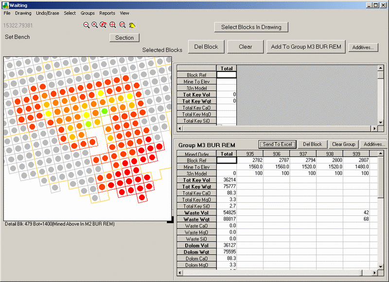
If a single block is selected with the right mouse key, a detail of the block is displayed as shown here: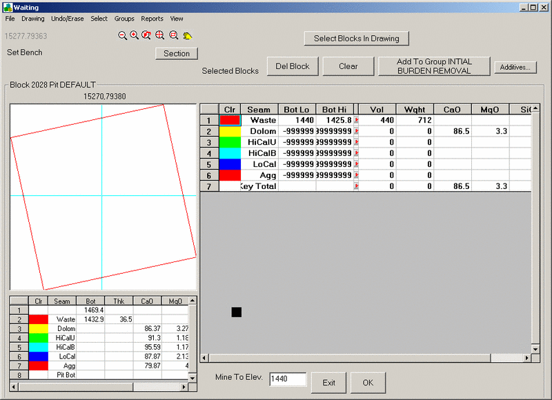

As the mouse is moved throughout the block, the detail data is shown in the spreadsheet in the lower left. That data reflect the values where the mouse lays in the block on the drawing. The total block data is shown in the right spreadsheet. The Exit button cancels the selection, and the OK button adds the block to the temporary list. (Optionally the block seams to mine, or the elevation to mine to is set as explained in later sections.)

Real-Time Block Data Feedback:
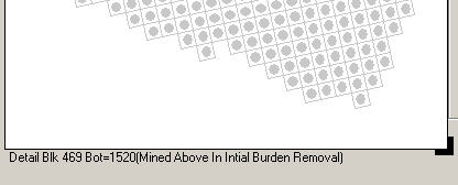
As the mouse is moved the text under the drawing gives basic feedback on the block. The data shows the bottom elevation of the topmost un-mined block the mouse is over. It also shows the group of the last mining that occurred in the block above.

Optional Real-Time Block Data Feedback:
By Selecting the Drawing pulldown > Block Realtime On/Off, a small chart appears under the drawing showing the breakdown of the block the mouse is over such as. The values change as the mouse is moved.

Locating Selected Blocks:
After blocks are selected, they may seem difficult to locate. So, the spreadsheet has some special actions that allow you to find a block on the drawing.

Option 1: Place the cursor in row 1 of any block in either spreadsheet. Right-click the mouse. The drawing will shift so that the particular block is centered on the screen.
Option 2: Place the cursor in any row other than 1 of any block in either spreadsheet. Right-click the mouse. The drawing will highlight the block similar to:

The highlight remains on until another block is selected.

Changing Analysis Screen Appearance

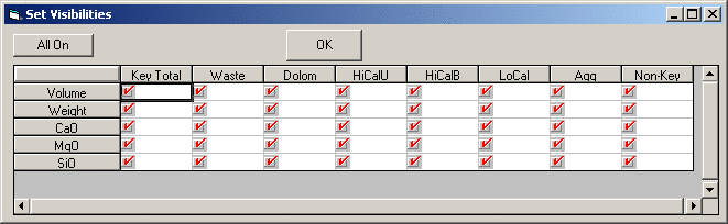
Manipulating The Spreadsheet Data Visibility: By default the spreadsheets show all data for all seams. In addition, the total Key data is shown at the top of the spreadsheet, and the total Non-Key data is at the bottom. The left column in the spreadsheet is the total of all blocks in the spreadsheet. The following example shows the layout:

The data visibility can be set with the pulldown menu View> Set Quality Visibility. The following grid appears to turn particular data on/off:

Lock the Key Data Display: The Key data can be prevented from scrolling in the spreadsheet with the pulldown menu View> Freeze Key Info.
Turning Pit Areas On/Off From Visibility: The pulldown menu View will contain the name of each Pit. Clicking on the name of each pit with turn the areas on/off in the drawing.
Colorizing Blocks: Blocks can be colored in various ways using the pulldown Menu Drawing> Colorize>
By Bench: Each level of mining is assigned a new color. A legend appears on the right edge of the drawing.

Best to Worst: This section shows suitability of mining on a graded scale. The following menu appears:

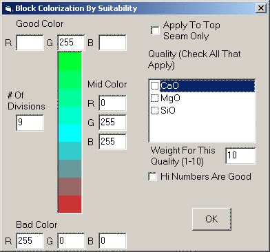
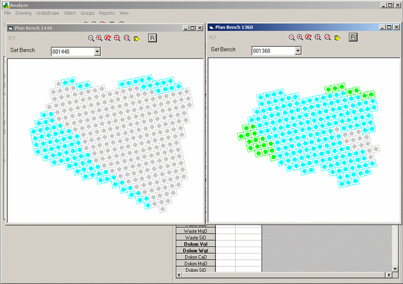
The left side of the screen allows you to set the number of colors, and the red, green, blue components of the good, bad, and mid-range colors. The right side of the screen allows selection of the qualities to consider. Turning on the checkbox activates that quality in the weighting. The Weight For This Quality box allows the user to weight a particular quality greater or lower than others in the analysis. The value has no application for a single quality. The Hi Numbers Are Good check box allows the user to specify whether the best value of the quality is a high or low number. The following is an example of the result with 2 qualities, equally weighted. Gray blocks are areas with no quality information to weight.

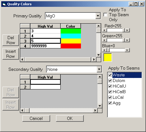
By Qualities: This section shows colors by a primary and optionally a secondary quality. A menu will appear similar to:

The primary quality is selected in the top box. In this case, MGO was selected. Then a series of breaks was entered into the top spreadsheet. The example shows 3, 4, 5, and 9999999. This would equate to zones of : 0-3, 3-4, 4-5, 5 and up. When the cursor is on a particular row, slide the Red, Green And Blue sliders to obtain a color. Double click in the preview color box under the sliders to set that color to that row.

The secondary quality will be used (if included) to set shades of colors between the two primary colors ranges. Set the applicable seams (materials or strata) and press OK. Each block will be displayed in its own color, for the weighted total of the selected materials.

Additional Plan Views: Additional plan view windows can be opened using the pulldown menu Drawing> New Plan View. The windows are designed to show a single mining elevation level (bench) at a time. The windows float. That is, they disappear behind the main form when it is active, but remain in the task bar and can be brought to the top by clicking there. The bench elevation to show is set in the pulldown at the top. Below is an example where one window shows the blocks at elevation 1440, and the other at 1360. The windows do not update automatically with mining changes (a speed consideration). Use the R button to refresh them.

Section View: A section view window can be opened using the pulldown menu Drawing > Section View. The window is designed to show a single east-west section view. The window floats like the additional plan views. Once the Section view is activated, click the Section button above the main drawing. Click any point on the drawing. Return to the Section view and zoom extents.

Limiting Mining In Blocks:

Limiting the Mining of the Block By Elevation: The second row of the temporary spreadsheet is labeled “Mine To Elev” By default, when a block is picked, this value is set to the bottom elevation of the block. If the value is changed to a value higher than the bottom, the block is reanalyzed and the data updated. Setting it to a value lower than the block has the same effect as mining the entire block.
Limiting the Mining of the Block By Material: Each material (strata) has a check box row in the spreadsheet. If that box is turned off, and the active cell changed, all materials below the one in question are turned off, the block is reanalyzed and the data updated. Similarly, if the cell is turned on, all materials above it are turned on, the block is reanalyzed and the data updated.
Limiting the Mining of the Block By Material On the Entire Temporary Spreadsheet: Double-clicking the left-most (gray) column in any row with check marks, changes all blocks in the temporary spreadsheet at once.
Limiting the Mining of the Block By Material Before Selecting: To mark the strata to be mined before the blocks are selected, use the menu File pulldown, >Set Lowest Mined Strata. Set the lowest strata to mine and press OK. As the blocks are selected, the materials below the strata selected are marked as unmined.

Note: When a block is partially mined, and added to a group, the remainder of the block is still present for selection in the drawing. For example, if we mine two block, one to elevation 1460, and one through the ‘Waste’ seam. The drawing would appear as:

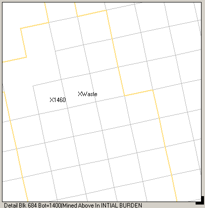
This text is only visible when the drawing is zoomed to a fairly tight scale. The next time we choose that block, the material mined previously will be not be shown, because it has already been removed from the block

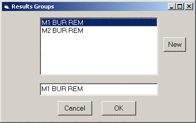
Groups: Groups are named collections of mined blocks. One group is active at a time. The name of the group active is in bold text in the lower spreadsheet. The button about the temporary spreadsheet also will be labeled “Add To Group <Name>” Where name is the group that the temporary blocks will be added to when pressed. To edit the group list, either use the pulldown menu Groups> Add New Group, or simply double-click the name of the group in the lower spreadsheet. A screen will appear:

Double-click any title to make the group the current group, and to edit its name in the lower box, or press the new button to add a new group and name it. When the OK button is pressed, the current group data is displayed. When a group is displayed, the drawing zooms to the group limits, and draws a yellow boundary line around the group such as:

Editing Block Data: If a cell is selected in the block, and the Del Block button is pressed, the block will be deleted from the group. The Clear Group button will delete all blocks.
Send To Excel: This button will dump the current group data to Microsoft Excel.
Undoing Actions: Each time a series of blocks is moved from the temporary spreadsheet to a group, a record of the transaction is made in the database. Using the pulldown menu Undo/Erase> Undo command will undo the last transaction record in the database. Using the pulldown menu Undo/Erase> Redo Last Undo will redo what was just undone. However, this is only usable once between transactions. Using the pulldown menu Undo/Erase> Erase Back To A Block # allows you to remove blocks from the mine plan back to the point a single block was added to a group. The block numbers are labeled in the top row of the group spreadsheet.
Analysis Reports: After a series or groups are mined, the summary report can show the totals of each group, and an overall total. Use the pulldown menu Reports> Summary Page to get the totals. An example is shown here:

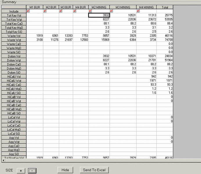
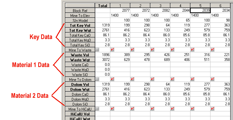
The check box at the top of each column includes or excludes the column from the total column. (The box must be changed and the cell exited before the totals update). The data can also be exported to Microsoft Excel with the Send to Excel option.

Pulldown Menu Location: Block Model
Keyboard Command: csbm