Prepare Value Block Model
This command makes a block model that represents
the profit of each block. . There are two options, to just Enter
the Economic Parameters or to Read Grid Parameters File. A 3-D
fixed block model is used for computerized optimization techniques.
Carlson defines a block model with a block file (*.blk) and top
elevation grid file, bottom elevation grid file and grid files with
grade parameters for each layer. The block dimensions are dependent
on the physical characteristics of the mine, such as pit slopes,
dip of deposit and grade variability as well as the equipment
used. The center of each block is assigned, based on drill
hole data and a numerical technique, a grade representation of the
whole block. Carlson uses inverse distance method, 3D Kriging, and
discrete method to estimate grades for each block. A block model
can be created using the “Make Block Model” (Command: blkmodel) or
the Input-Edit Block Model commands from “Ore” menu.
A value block model consists blocks with profit
($/block) values associated with them. These profit values are
calculated based on the grade values of the blocks. The command to
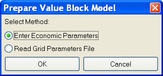
make value block model starts with a dialog to choose Carlson block
model to process. The first dialog is for selecting the Method for
Preparing the Value Block Model. The first option, to Enter the
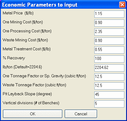
Economic Parameters brings up the following window where the final
Ore or Metal Price is set in $/lb for all the key ore.
 The second option, to Read
Grid Parameters File, brings up the following window where price
for each grade ($/lb) appears just as it is entered in the Grade
Parameters file GPF.
The second option, to Read
Grid Parameters File, brings up the following window where price
for each grade ($/lb) appears just as it is entered in the Grade
Parameters file GPF.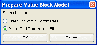
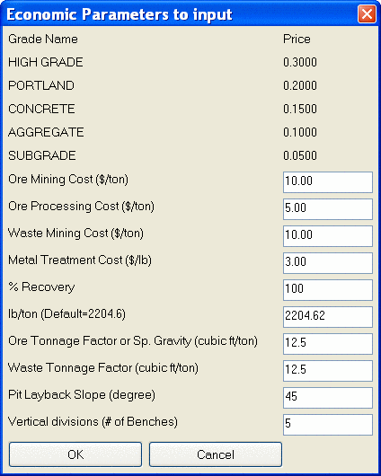
Each of the input parameters are described
below:
- Metal Price ($/lb): The price obtained for a lb of final
product
- Ore Mining Cost ($/ton):
Cost associated with mining a
ton of ore
- Ore Processing Cost ($/ton):
Cost associated with processing
a ton of ore
- Waste Mining Cost ($/ton):
Cost associated with mining a
ton of waste
- Metal Treatment Cost ($/lb):
Cost associated with treatment
of a lb of ore
- % Recovery: The fraction of contained product recovered
during processing
- lbs/ton (Default=2204.6):
Factor used to convert tons into
lbs, 2204.6 for long ton and 2000 for short ton
- Ore Tonnage Factor or Sp. Gravity
(cubic ft/ton): Density of the
ore
- Waste Tonnage Factor (cubic ft/ton):
Density of the
waste
- Pit Layback Slope (degree):
Overall slope of the pit
highwalls
- Vertical divisions (# of
Benches):This is the number of benches allowed for the
surface pit
Using the above input values, first the Net value/lb for ore is calculated as
follows:
n= Netvalue/lb = (Metal Price – Treatment cost) *
recovery/100$/lb
c = ore mining cost + ore processing cost + waste mining cost
Then calculate the Cutoff grade: x %
(x/100) * lb/ton * n = c
And Mill cutoff grade: y%
(y/100) * lb/ton * n = (c – Ore processing cost)
Now we already know the block size (height, width and length) so we
can calculate its volume V = h*w*l ft3. And with tonnage factor we
can calculate tons/block = Tb = V/tonnage factor. Then Profit
associated with each block is calculated based on its Grade value
that is read from GPF file:
For any block
(a) if Grade is less than (<) y
- Revenue = 0
- Cost = Tb * Waste Mining Cost
- Profit = Revenue – Cost
(b) if Grade is greater than ‘y’ but less than
‘x’
- Revenue = Tb * (ore grade of the block/100) * (Metal Price *
lb/ton)
- Cost = Tb * (Ore Mining Cost + Ore Processing Cost + Ore
Treatment Cost)
- Profit = Revenue – Cost
(c) if Grade is greater than “x”
- Revenue = Tb * (ore grade of the block/100) * (Metal Price *
lb/ton)
- Cost = Tb * (Ore Mining Cost + Ore Processing Cost + Ore
Treatment Cost)
- Profit = Revenue – Cost
The blocks with positive Profit are treated as profitable block and
the profit value associated with each block is saved in new BLK and
GRD files. Then the Lerchs Grossmann Algorithm is used on this
Economic Value Block Model to calculate the optimum pit. If the
grade block model has more than one attribute (grades) then
economic parameters are read from gpf file, otherwise economic and
physical parameters are entered directly to create the new value
block model. A surface grid file is read to create the surface of
the new block model. All the blocks that lie between surface grid
and top elevation of the grade block model are treated as waste
blocks i.e. grade is assigned to zero for those blocks. The number
of blocks and size of blocks in the new block model are
calculated based on the physical parameters, pit layback slope
angle and number of vertical divisions. The block values (grade)
for the new block model are estimated using the original block
model. Profit (dollars/block) associated with each block is
calculated based on its physical and economical parameters. The
blocks with positive profit are treated as ore block. The Value
Block Model is saved as a new Carlson block model file
(*.blk). There are file selection windows to first select the
existing block model (BLK file), the surface Topo grid file and the
new Value Block Model to write. The final step is to write out the
Value Block Model that may be used in other routines, such as
Optimized Pit Design. Keyboard
Command: mkvalblkm
Pull-down Menu Location:
Block Model
Prerequisite:
Need a BLK model file, a topo
grid file and optionally a GPF grade parameter file.