Optimized Pit Design

This command uses the Lerchs-Grossmann Algorithm (LGA) to determine the optimized minable pit. Determining the optimum ultimate pit of a mine is the base of mine planning. The optimum ultimate pit of a mine is defined as the "pit shell contour", which is the result of extracting the volume of material that provides the total maximum profit while satisfying the operational requirements of safe wall slopes. The ultimate pit limit gives the shape of the mine at the end of its life.  Usually this contour is smoothed to produce the final pit outline. Optimum pit design plays a major role in all stages of the life of an open pit:

• At the feasibility study stage when there is a need to produce a whole-of-life pit design;
• At the operating phase when pits need to be developed to respond to changes in metal prices, costs, ore reserves, and wall slopes; and
• Towards the end of a mine’s life where the final pit design may allow the economic termination of a project.

At all stages there is a need for constant monitoring of the optimum pit, to facilitate the best long-term, medium-term and short-term mine planning and subsequent exploitation of the reserve.  The optimum pit and mine planning are dynamic concepts requiring constant review.  Thus the pit optimization technique should be regarded as a powerful and necessary management tool.  Further, the pit optimization method must be highly efficient to allow for an effective sensitivity analysis. The ultimate pit limit problem has been efficiently solved using the Lerchs-Grossmann graph theoretic algorithm.

Lerchs-Grossmann Algorithm for ultimate pit design
Following is a detailed description of the internal workings of the algorithm.

1. Define a cutoff grade for the mine.

2. Consider the physical location of the Blocks.

3. Calculate the average grade value (profit or loss) associated with each block. This is done with the command Prepare Value Block Model.

4.  Considering that overlying blocks must be removed before mining the lower blocks, find possible connections of blocks from lower level to upper levels.

• 1-5 pattern (at least 2 common vertices between lower and upper blocks)
• 1-9 pattern (at least one common vertex between lower and upper blocks)

5. Imagine a dummy root (X0) connected to all the blocks with arcs and form a tree T0, assign M (profit) to all the arcs.

6. Assign direction to arcs

• Plus – if arc is directed away from the root.
• Minus – if arc is directed towards the root. (Note: Initially all the arcs will be in “Plus” direction.)

8. Divide all the arcs into two groups “Y” and “X-Y”.

• “Y” – contain all the arcs labeled “Strong”.
• “X-Y” – contain all the arcs labeled “Weak”.

9. Find all possible directed arcs from group “Y” to “X-Y”, if there are no possible arcs from group “Y” to “X-Y” the tree has normalized and the blocks belonging to group “Y” will be mined to give maximum profit, else go to next step.

10. Choose any possible arc (Xk, Xl) such that Xk belongs to group “Y”, and Xl belongs to group “X-Y”.  Determine Xm, strong root of Xk connected to dummy root X0.

11. Drop arc (X0, Xl) and connect (Xk, Xl) and construct a new tree Ti.

12. Update weights according to following transformation

• For an edge ei on the chain [Xm ……Xk] => Mnewi = Mm - Moldi
• For edge (Xk, Xl)  Mk = Mm
• For an edge ej on the chain [Xl………..Xp, X0] => Mnewj = Mm+Moldj

13. Go to step 6 and repeat the procedure again.

This application is developed using a modified version of LGA. Here we consider only two consecutive branches at a time and normalize them and update the weights or values associated with the each node in the grid.

Ultimate Pit and Cyclic Production Report Generation
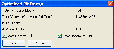
A pre-existing value (profit) block model is selected to process form this command. The block model is processed using Lerchs Grossmann Algorithm (LGA) to find the Ultimate Optimum pit. There are two methods to determine the ultimate pit. The first method will use the LGA For All Levels. This brings up the second dialog box, where the Total number of blocks is displayed. Below that is the Total Volume, and the breakdown of number of Ore Blocks and # of Waste Blocks. There are two output methods here. Save the Ultimate Pit grid, which will prompt for a new BLK file to save out, and save the Bottom Pit Grid, which will prompt for a new grid file to create, of the bottom of pit surface.

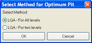
LGA-For All Levels takes all the benches into account at the same time and if there exists an optimum pit, it will find it. It takes care of the constraint that the algorithm for two levels uses. As this one is a iterative process it takes a little long to find the optimum pit if we have large block model.

LGA-For Two Levels will bring up the next dialog window.

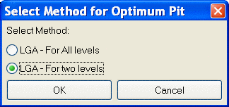
LGA-For Two Levels considers only TWO BENCHES at a time, starting from top to bottom. Lets say we have 5 benches in our block model, it takes into consideration bench 1 (top bench)  and 2 and finds the optimum pit and updates the profit values of them. Then it takes bench 2 (this bench has updated weights or profit values) and 3, and repeats the same steps for the rest of the benches. The main constraint with this algorithm is that if you more than 2 benches of over burden it will not work.

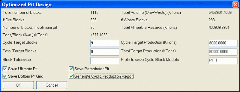
The following items are shown at the top of the dialog. These are calculated using the LGA on the predefined Value Block Model.

• Total number of blocks
• Total Volume (Ore+Waste) (KTons)
• # of Ore Blocks
• # of Waste Blocks
• Number of blocks in the optimum pit
• Total Mineable Reserve (KTons)

The next 6 items are input values used for creating a cycle or schedule report.

• Cycle Target Blocks: This is the number of blocks that can be mined per cycle period.
• Cycle Target Production (KTons): These are the tons that can be produced per cycle period.
• Total Target Blocks: This is the total number of blocks to be mined in all the cycle periods.
• Total Target Production (KTons): These are the total tons to be mined in all the cycle periods.
• Block Tolerance: This is the tolerance allowed per cycle. +/- this many blocks per cycle period.
• Prefix to save Cycle Block Models: Enter the prefix to assign to the output block model.

The final four check boxes are options to create the output files. the Save Ultimate Pit creates an output BLK file. The Save Remainder Pit is the pit left by mining the total targeted blocks, also saved as a BLK file. All cyclic pits (block models) are saved with given prefix and a cyclic production report is generated showing production and economic details of all the cycles. The Bottom pit grid file can only be saved with save ultimate pit and save remainder pit options selected. The Cyclic Report gives the production per cycle defined.

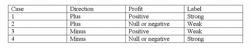
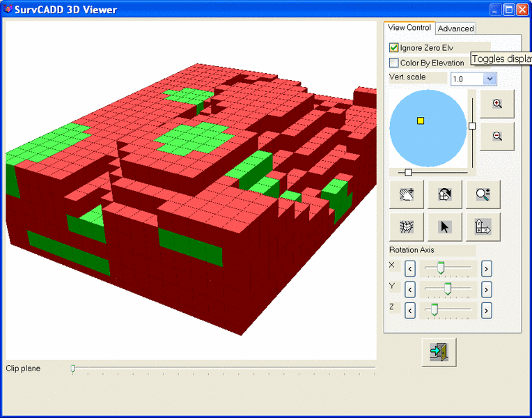
The values of the ULTIMATE PIT BLK file should be the same as it was in the value block model except for the blocks which has to be mined, it assigns NULL value to the blocks that are to be mined, so that we can visualize what the blocks are that are in the group that is to be mined. The rest of the blocks will have either +ve or -ve values based on whether its a Profit Block or Non-Profit block.

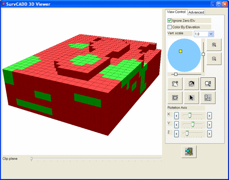
Here is an example of a limestone quarry. Consider the two views of the geologic block model. With the lowest grade removed (yellow), the highest grade, green can be seen. After creating the Value Block Model and generating the Ultimate Optimized Pit, these next views show where it can be mined by running the LGA on the Value Block Model. The first shot is of the value block model. Make a new Grade Parameter File to show Profit and Loss. In this case, Red is Loss, and Green is Profit, but there may be numerous intervals. Then use the Block Model Viewer to see the "before and after."

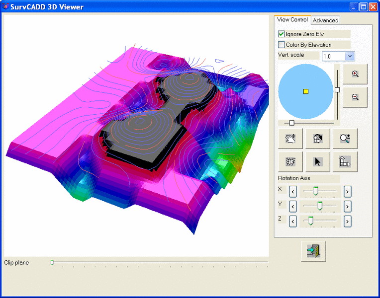
The final shot is of the output grid file representing the ultimate pit. The original contours are shown above the final grid surface for comparison.

Limitations
There are a few limitations that need to be considered when creating the optimum pit at this time. Future releases might look into some of these.

• The variation in mining cost with depth is not considered.
• Only one layback slope angle can be assigned to all the benches.
• On large models, the speed will be very slow.
• It cannot handle a block model with three benches (layers) of overburden or three consecutive waste benches (layers).
• Sometimes algorithm may not converse for desired number of blocks in that case changing block tolerance might help.
• All cycle block models produced cannot be viewed in 3D viewer at the same time.
• The dimensions and starting coordinates should match in surface grid file and rest block model grid files.

Pulldown Menu Location: Block Model
Keyboard Command: bestpit
Prerequisite: Need a value block model