This tutorial steps through examples of how to handle outcrop and subcrop conditions on several examples involving ridge top mines as well as sub-cropping reserves. Accurately locating the crop is one of the first things the planner needs for laying out a mine. Carlson automatically detects the location of the crop within the Surface Mine Reserves command. Volumes will never be calculated from above the ground surface. The advantage of the Draw Outcrop routine is that it allows the user to witness where the program is interpreting outcrops and subcrops. It is also useful in establishing a starting perimeter for pit layout. Outcrops are automatically calculated and drawn using Draw Outcrop command under StrataCalc on the fly directly from the drillhole data, or from pre-calculated grids.
For Generating Outcrops Directly from Drillholes ("On the Fly")
For Generating Subcrops
Outcrop Procedure
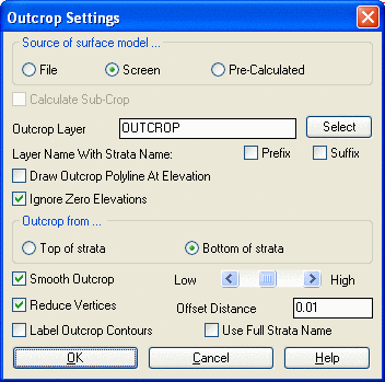
Select Draw Outcrop in the StrataCalc menu. Fill in the Outcrop
Settings dialog box. The user can specify the source for surface
topography (grid file or screen selection) and what layer to store
the outcrop in when it is drawn. The user normally will use the
settings as shown in the dialog box below with one exception. The
offset distance could be set to 0.1 to 1.0 ft to reduce the
vertices in the outcrop when drawn. Otherwise, the polyline for the
outcrop will contain an unnecessarily large number of points.
Command: outcrop
Select surface entities & at
least 3 drillholes
Select objects: Specify opposite corner: 111 found
Use drillhole surface elevations in surface model
[Yes/<No>]? Y
if they match the contours, otherwise N
Reading points ... 79695
Ignored 562 points with zero elevation.
Ignored 36 duplicate points.
Intersections found 80377
Pass> 10 Null Z values left> 0
Finding splits ...
Finding pinch out ...
Calculating seam stacking ...
Output grids for strata and surface [Yes/<No>]?
NThe files may be saved
out for other uses. No is the typical response.
Choose modeling method
[<Triangulation>/Inverse
dist/Kriging/Polynomial/LeastSq]?
Apply global trend to strata extrapolation [Yes/<No>]?
Y
Use Triangulation Subdivision [Yes/<No>]? N
Triangulating points ... 5
Assigning grid values> 98400
Pass> 282 Null Z values left> 0
Contouring elevation 0.0
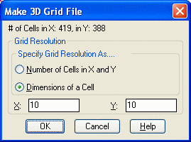
Inserted 348 contour vertices. Complete the Make Grid File dialog box. The user may select the total number of rows and columns or the grid spacing pattern option. The program creates the grids "on the fly" from the drillhole data.
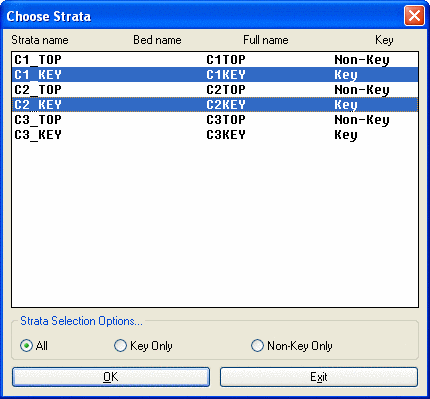
 Select the
preferred method. Once the gridding method is selected the
Choose Strata dialog box appears. Choose the strata to
process. Each strata can be gridded using independent gridding
algorithms. If Inverse Distance or Least Squares was selected as
the gridding method, when the strata is selected, the user is
prompted for the power to be used in the algorithm. Once the power
is entered, assuming Inverse Distance or Least Squares is the
selected method, the user is prompted for other strata to be
processed. The user can select any number of strata to be processed
by holding down the CTRL or SHIFT buttons.
Select the
preferred method. Once the gridding method is selected the
Choose Strata dialog box appears. Choose the strata to
process. Each strata can be gridded using independent gridding
algorithms. If Inverse Distance or Least Squares was selected as
the gridding method, when the strata is selected, the user is
prompted for the power to be used in the algorithm. Once the power
is entered, assuming Inverse Distance or Least Squares is the
selected method, the user is prompted for other strata to be
processed. The user can select any number of strata to be processed
by holding down the CTRL or SHIFT buttons.
Outcrop lines are produced on elevation zero. To raise the outcrop to the surface, use the command 2D to 3D Polyline by Surface Model command under 3D Data in the Carlson Civil. This uses the surface model as the basis for assigning elevation to the outcrop polyline.
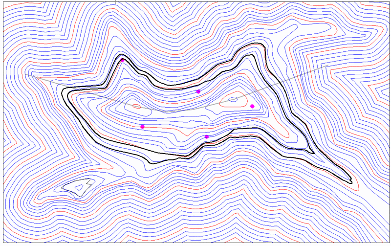
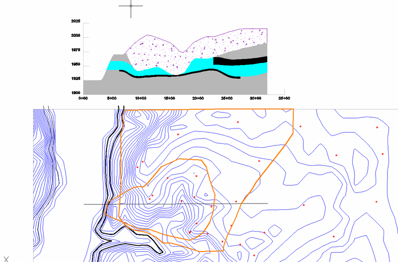
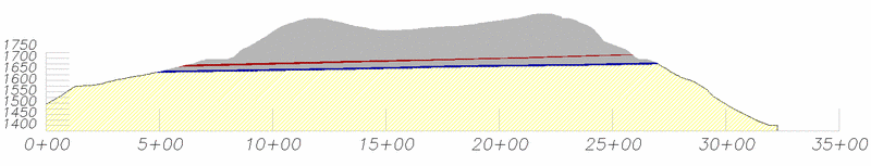
Making Fence Diagrams
As a way to verify the location of the outcrop or make a graphic
presentation, a fence diagram can be created using the Fence
Diagram command under Stratacalc. Fence diagrams are useful for
presenting geologic data as well as verifying the proper location
of seams and their burden. Shown below is a fence diagram taken
from the line drawn from west to east through the outcrops on the
hill.
 Fence
Diagram Procedure and Prompting:
Fence
Diagram Procedure and Prompting:
Command: fence
Select polyline to pull fence diagram
from: Pick the polyline to get the fence from
Use drillhole surface elevations
in surface model [Yes/<No>]? N
Select surface entities and at least 3 drillholes. Select
the drillholes and surface contours
Select objects: Specify opposite
corner: 112 found
Reading drillhole 5
Finding splits ...
Finding pinch out ...
Calculating seam stacking ...
Ignore zero elevations [<Yes>/No]? Y
Reading points ... 79695
Choose modeling method [<Triangulation>/Inverse
dist/Kriging/Polynomial/LeastSq]? I Choose a modeling method you
prefer.
Use inverse distance to which
power [First/<Second>/Third/Other]? S
Use elliptical inverse distance
[Yes/<No>]?
Calculating grid by inverse distances 98456...
Bottom elevation of grid <1650.00>: 1400
Pick the lower left corner for the diagram: Pick an open
area in the drawing for the lower left corner of the diagram.
 Layer Settings button
can be used to set layers for the different components of the fence
diagram.
Layer Settings button
can be used to set layers for the different components of the fence
diagram.

Using Surface Reserves to Check the Outcrop
Volumes
To prove that Carlson honors the outcrop in its calculations,
layout a rectangular polygon that overlaps the outcrop area. If
Surface Mine Reserves recognizes the seam crop, then the area of
the seam will be less than the area of the perimeter, and the upper
seam crop area will be less than the lower seam area. It calculates
reserve areas and handles outcrops automatically. Higher surfaces
(the topography in this case) are the limiting factors. Volumes
will never be calculated above the next surface up.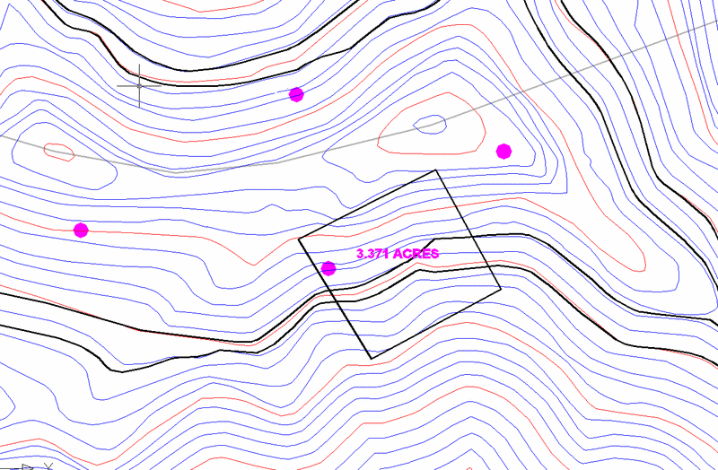 The area
of the perimeter is shown as 3.371 Acres, some of it within the
area of coal, and some outside. Run the Surface Mine Reserves
command using the perimeter to get the tons and acres of coal. A
typical report from the Surface Mine Reserves command under
StrataCalc is shown below. Reports are user-defined in the Report
Formatting dialog box.
The area
of the perimeter is shown as 3.371 Acres, some of it within the
area of coal, and some outside. Run the Surface Mine Reserves
command using the perimeter to get the tons and acres of coal. A
typical report from the Surface Mine Reserves command under
StrataCalc is shown below. Reports are user-defined in the Report
Formatting dialog box.
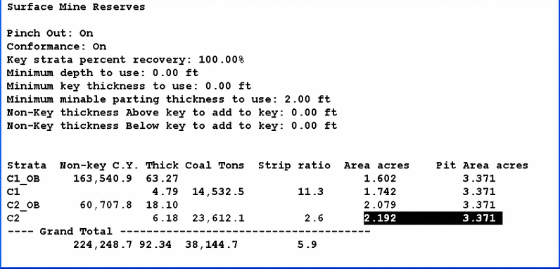
As the report indicates, Carlson recognizes the limits imposed
at the outcrop. It successfully truncates the seam at the outcrop
and reports the included area between the crop and rectangle.
Notice the C1 has less acres than the C2 because it crops out
higher on the slope. the C2 shows 2.192 Acres compared to the full
3.371 Acres of the polygon. The Pit Acres are reported as an
available option in the Formatter.
In topographic situations similar to the one shown in this example, for coal, the user will have to deduct from the mineable reserves for crop loss. Crop loss sometimes runs 10' to 15' vertically. The coal in this zone is usually oxidized to such an extent that the BTU is so low and the ash is so high, the coal cannot be sold for steam product, and chemistry is so poor that it cannot go for metallurgical product either. Oxidized coal is treated as overburden.
Using Outcrops for Laying Out
Pits
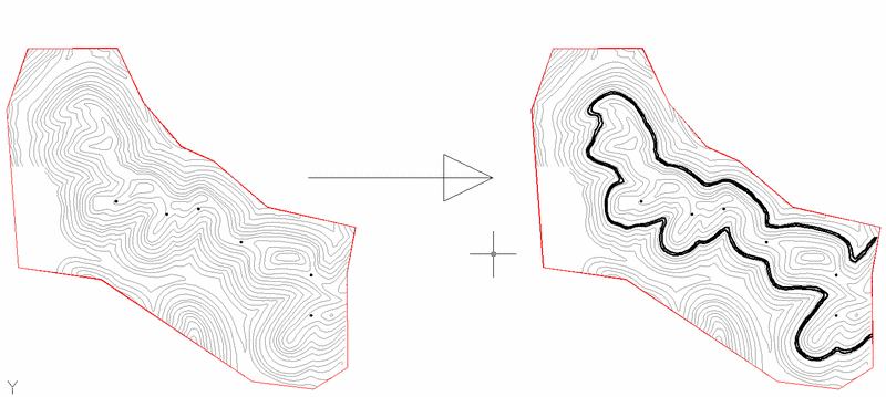
In the example below, the outcrop was used to define the limits of
the surface mining pits. The outcrop defined the limits of mining
on each side of the pit. The direction of mining was input as part
of the pit layout routine. The example below shows the Pit Layout
By Advance command executed on the closed polylines.First,
create a close polyline of the outcrop/mine boundary. Use the
command Draw-Boundary Polyline and pick inside the ridge/outcrop
lines to get a new interior polyline. You can also use AutoCAD's
BPOLY command. Then, draw a direction line down the ridge to assign
direction. Pits will be cut perpendicular to this line.
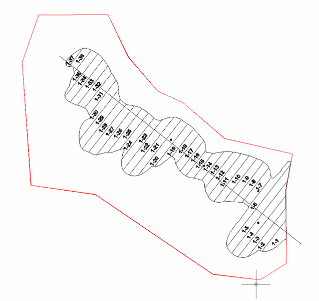
Pit Names, Labels, and Identify Pit Names
Since the process of laying out pits using the Pit Layout By
Advance option gives the pits a name, a discussion of naming and
labeling procedure is helpful at this point. After the pits are
drawn, there are two methods to draw the pit name labels. Go to
Label Pit Polylines or Pit Label Formatter. Identify Pit Polylines
allows the user to see the Pit Names when the labeling option was
not selected.
Subcrop Procedures
Subcrops occur where the unconsolidated material (could be glacial
till or a channel deposit) has eroded out the key seam below the
surface. Subcrops differ from pinchouts, in that unlike pinchouts,
which can occur anywhere below the surface, lower strata being
eroded by the unconsolidated material cause subcrops. Unlike
outcrops which can be created "on the fly" from drillhole data,
subcrops are calculated from grids. To calculate subcrops, the user
must have the surface grid, thickness grid of the unconsolidated
material, and bottom elevations of the strata to test for
subcropping. In addition to the gridding algorithms, the user can
specify strata limit polylines to override the natural mathematical
interpretation of the data. When Carlson calculates the subcrop it
starts from the surface and works down through the grids. If an
upper grid has a lower elevation lower than that of a lower grid,
the elevation of the upper grid is set to the elevation of the
lower grid. This leads to a zero thickness in the lower grid, or a
subcrop. Select the File option to begin calculating the subcrop.
Carlson allows the user to calculate the subcrop from a
pre-calculated grid or directly from the drillhole data.
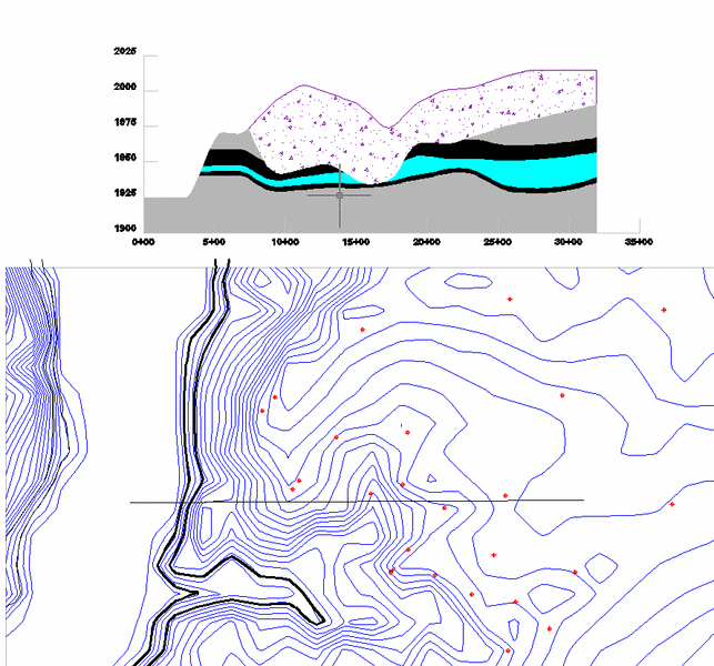
This example was created by making strata grids from the drillholes. Put them in the PreCalc grids file and then generate a Fence Diagram. The outcrop coincides with the outcrop lines in plan view on the hill side. Notice how the glacial till is subcropping the upper coal seam and the parting.
Strata Limit Polylines
Using the same example
for the Subcrops above, we will now create Strata Limit Polylines
for both the coal seams and the parting. They must be drawn in plan
view, then named with Name Strata Limit Polylines. Strata Limit
Polylines must be turned on under Configure , Mining Modules. There
are options to use them, and to automatically select them. The
orange lines are limit lines. The interior line is an Exclusion for
the upper coal seam. The outer line is an Inclusion for the lower
coal seam. Volumes will be calculated accordingly with Surface Mine
Reserves.