This tutorial is divided into two lessons covering the process
of reducing and adjusting raw survey data into final
adjusted coordinates, using the SurvNET program. The tutorial will
describe the reviewing and editing of the raw data
prior to the processing of the raw data. Next, the least squares
project
settings will be described, and then the final report generated from
the least squares processing will be be reviewed. This tutorial will
review both a total station only project, and a project that combines
both total station and GPS vectors.
The raw data files associated with this tutorial is located in the Carlson2007\Data folder, under the installation
folder on your
computer (example: \Carlson2007\DATA).
2 The first
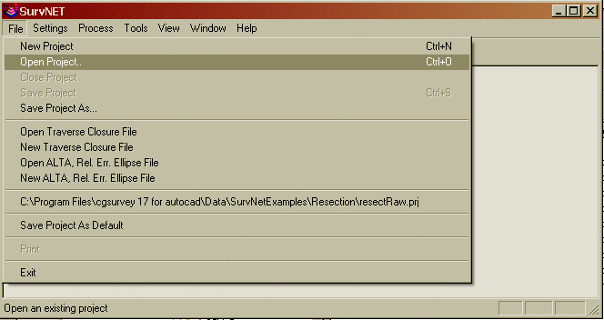
step is to open an existing project
or create a new project. We will open an existing project. Choose Open Project from the
File menu. Navigate to the \Carlson2007\DATA\ folder and open the
SurvNetTut01 project.
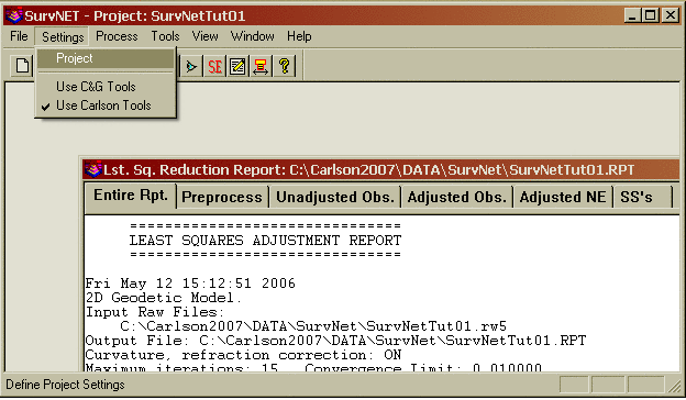
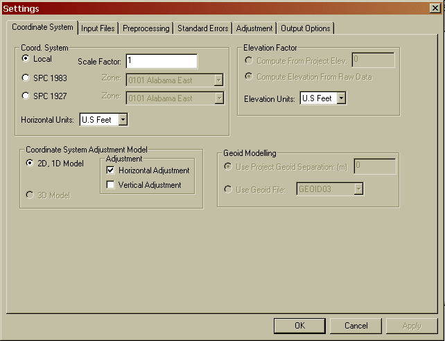
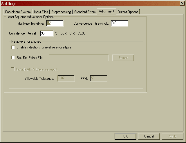
3 Learning the meaning and implications of the different project settings is the most critical initial step in learning how to use SurvNET. Let's review the different project screens. Choose Project from the Settings menu.
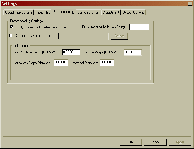
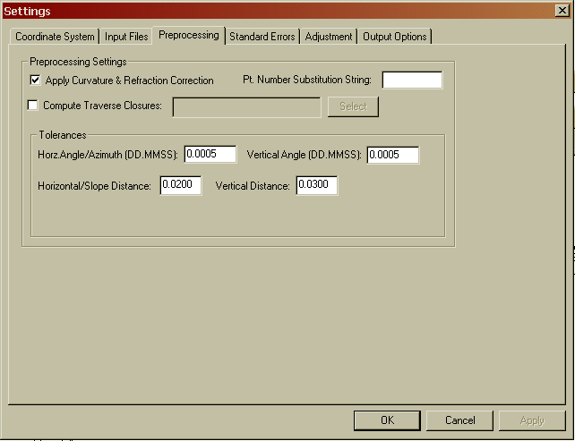
6 Choose the
Preprocessing tab to review the least squares
preprocessing settings. For the purpose of this tutorial, the
Preprocessing settings should look as
follows before proceeding to the next step. Preprocessing
consists of reducing and averaging all the multiple measurements,
applying curvature and refraction correction, reducing the measurements
to grid if appropriate, and computing unadjusted traverse closures if
appropriate. Much of the data validation is performed during the
preprocessing step.
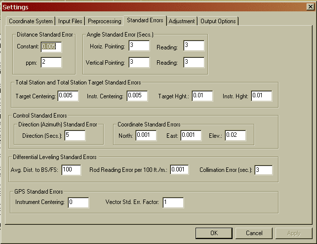
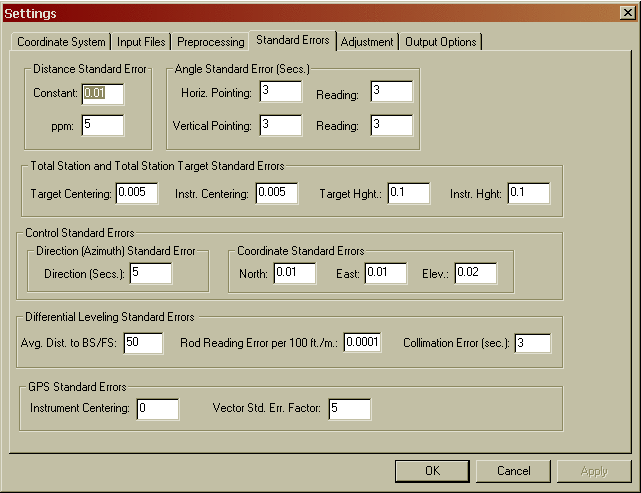
7 Choose the Standard Errors tab to review the standard error settings. The standard error settings should look as follows before proceeding to the next step. Standard errors are an estimate of the different errors you would expect to obtain based on the type equipment and field procedures you used to collect the raw data. For example, if you are using a 5 second theodolite, you could expect the angles to be measured within +/- 5 seconds (Reading error).
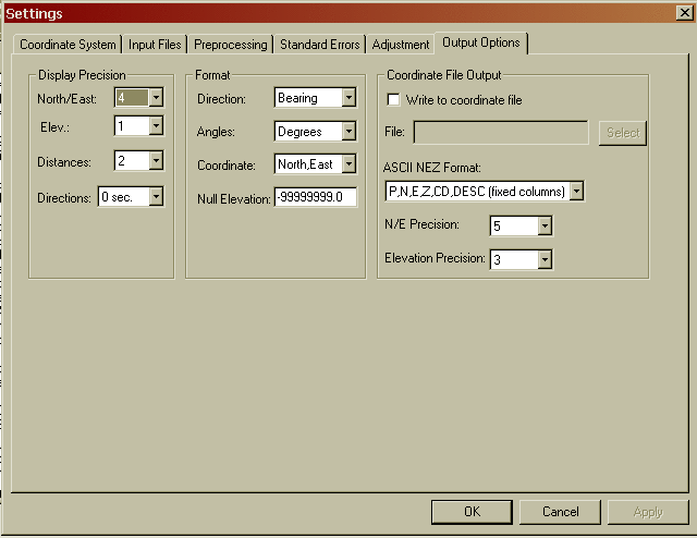
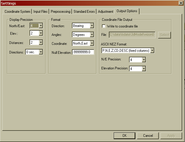
9 Choose the
Output
Options tab to review the output
settings. For the purpose of this tutorial, the Output Options settings
should look as follows before
proceeding to the next step. These settings apply only to the output of
data to the report files. These settings do not affect
computational precision. Press OK to return to the main SurvNET screen.
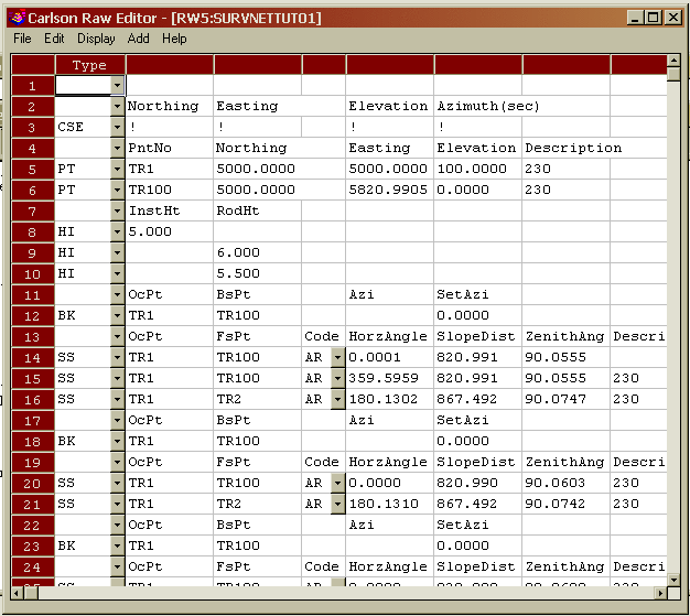
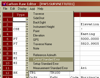
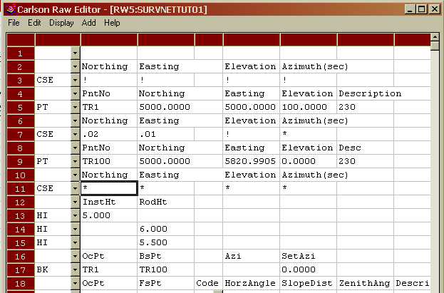
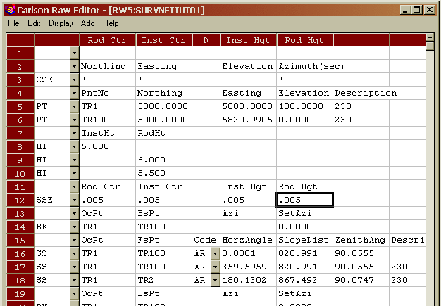
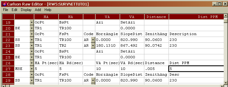
10 To review or
edit
the raw data, choose the Edit Raw
Files command from the Tools menu.

12 After exiting
the
raw data editor, we are ready to perform the least squares
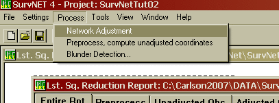
adjustment. From the Process menu, choose the Network Adjustment option.

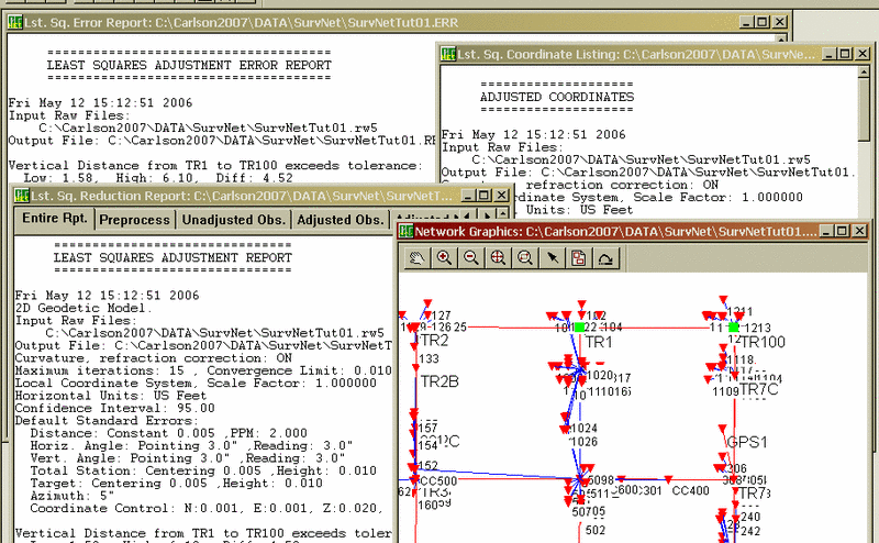
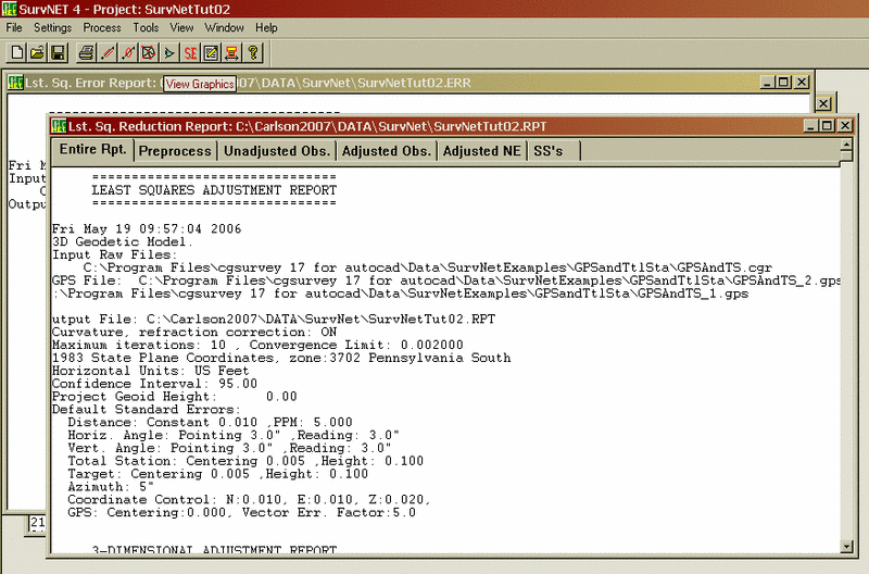
The
least squares adjustment is performed,
and the results from the adjustment are displayed. If the solution
converged correctly, the report should
look similar
to the following window. If there were errors or the
solution did not converge, an error message dialog will be generated.
If
there are errors, you will need to return to the raw
data editor to review and edit the raw data. Since the tutorial example
should have converged, we will next review the reports
generated by the least squares adjustment. There are four windows
created by the least squares program
during processing. These files include the .err file, which contains
any
errors or warnings that were generated during processing. The .rpt file
is the primary least squares report file summarizing the data and the
results from the adjustment. An .out file is created containing a
listing of the final coordinates. There is also a Graphics window that
is displayed. The graphic window is temporary and useful only for
seeing
the results of the survey. To bring up the Graphics window, choose
under the Window menu the Graphics command,
or click the View Graphics icon on the toolbar.
Relative Error Ellipses
Relative error ellipses are a statistical measure of the expected
error between two points. Regular error ellipses are a
measure of the absolute error of a single point. Some survey accuracy
standards such as the ALTA standards state the maximum
allowable error between any two points in a survey. Relative error
ellipses can give you this information. There is a more detailed ALTA
reporting feature in SurvNET. See the manual for additional information
on creating an ALTA report.
13 Press the Relative Error Ellipse toolbar icon button, or choose, off of the Tools menu, Relative Error Ellipse. Enter TR3 and TR7 in the From Pt. and To Pt. fields. Press OK to calculate. The dialog box should look as follows.
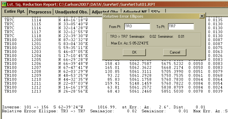
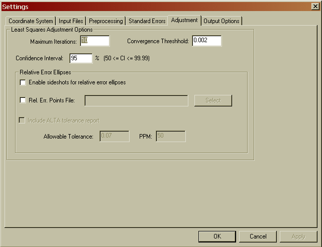
At the 95% confidence level there should only be around .02 feet of error between points TR3 and TR7. If you need to compute relative error ellipses for sideshots make sure the "Enable sideshots for error ellipse" toggle is set in the Adjustment tab of the Settings/Project dialog box.
14 In this section, the different sections of the least squares report are explained. If the Least Squares Report is not already showing, choose the Window menu and select the Least Square Report item. The report viewer has tabs to quickly access different sections of the report.
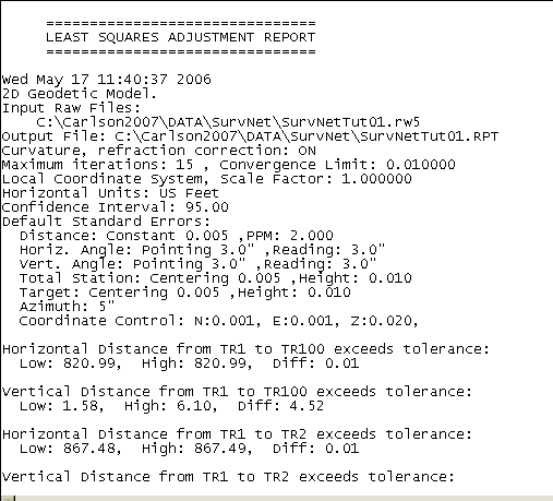
Preprocessing and Header Information
The following excerpt from the report shows the header information and the preprocessing results. The header information consists of the date and time, the input and output file names, the coordinate system, the curvature/refraction setting, maximum iterations, and distance units.
During the preprocessing process, multiple angles are reduced to a single angle and multiple slope distances, vertical angles, HI's, and rod heights are reduced to a single horizontal distance and vertical difference. During this process the horizontal angle, horizontal distance, and vertical difference spreads are computed. If the spreads exceed the tolerance settings from the Settings dialog box, then a warning message is displayed showing the high and low measurement and the difference between the high and low measurement.
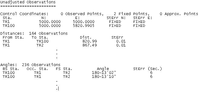
Unadjusted Measurements
The following excerpt from the report shows the unadjusted measurements. Measurements consist of some combination of control X, and Y, horizontal distances, horizontal angles, and azimuth measurements. These measurements consist of a single averaged measurement. For example, if multiple distances were collected between two points during data collection, only the single averaged measurement is used in the least squares adjustment.
Also, standard errors for the measurements are displayed in this section of the report. The standard errors are computed from the standard error setting in the Settings dialog box using error propagation formulas. The standard error of an angle that was measured several times would typically be lower than an angle that was measured only once.
If the data had been adjusted into NAD 83 coordinates both the
ground
distances and the grid distances would be displayed. The
grid, elevation, and combined factor would also be displayed in this
section of
the report.
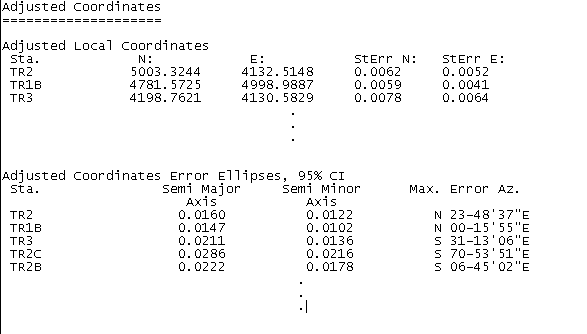
Adjusted Coordinates
The next section of the report shows the final adjusted coordinates. Additionally, the computed standard errors of the coordinates are displayed. If this project was reduced to NAD 83, the final latitude and longitudes are also displayed. Error ellipses computed to the 95 percent confidence interval are also displayed.
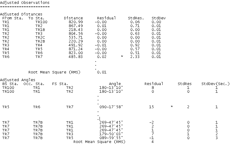
Adjusted Measurements
The following section from the report shows the final adjusted measurements. This section is one of the most important sections to review when analyzing the results of the adjustment. In addition to the adjusted measurement, the residual is displayed. The residual is the amount of adjustment applied to the measurement. The residual is computed by subtracting the unadjusted measurement from the adjusted measurement.
The standard deviation of the measurement is also displayed. Ideally, the computed standard deviation and residual and the standard error displayed in the unadjusted measurement would all be of similar magnitude. The standard residual is a measure of the similarity of the residual to the a-priori standard error. The standard residual is the measurements residual divided by the standard error displayed in the unadjusted measurement section. A standard residual greater than 2 is marked with an "*". A high standard residual may be an indication of a blunder. If there are consistently a lot of high standard residuals it may indicate that the original standard errors set in the Settings dialog box were not realistic.
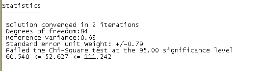
Statistics
The next section displays some statistical measures of the adjustment including the number of iterations needed for the solution to converge, the degrees of freedom of the network, the reference variance, the standard error of unit weight, and the results of a Chi-square test.
The degree of freedom is an indication of how many redundant measurements are in the survey. Degree of freedom is defined as the number of measurements in excess of the number of measurements necessary to solve the network.
The standard error of unit weight relates to the overall adjustment and not to an individual measurement. A value of one indicates that the results of the adjustment are consistent with the a priori standard errors. The reference variance is the standard error of unit weight squared.
The chi-square test is a test of the "goodness" of fit of the adjustment. It is not an absolute test of the accuracy of the survey. The a-priori standard errors which are defined in the project settings dialog box or with the SE record in the raw data file are used to determine the weights of the measurements. These standard errors can also be looked at as an estimate of how accurately the measurements were made. The chi-square test merely tests whether the results of the adjusted measurements are consistent with the a priori standard errors. Notice that if you change the project standard errors and then reprocess the survey the results of the chi-square test change, even though the measurements themselves did not change.
In our example the chi-square test failed at the 95% significant level. Our example failed the chi-square test on the low end, 52.6 is less than 60.5. Failing on the low end indicates that our data is actually better than expected compared to our a-priori standard errors. If we were to decrease the pointing and reading standard error in the Settings screen by 5-10 seconds we would probably pass the chi-square. Also notice that if you change the standard errors by only 5-10 seconds and reprocess the data the final coordinates will not change significantly.
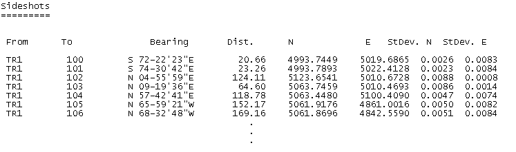
Sideshots
If the "Enable sideshots for relative error ellipses" is not set in
in the Adjustment screen of the project settings screen, sideshots are
computed separately after the adjustment is completed.
If the project had valid elevation benchmarks and measured HI's and rod heights the project could have been defined to adjust elevations. When using the 2D/1D least squares model the horizontal and the vertical adjustments are separate least squares adjustment processes. As long as there are redundant vertical measurements the vertical component of the network can also be reduced and adjusted using least squares. In the vertical adjustment, benchmarks are held fixed.
This is the final step in the adjustment. The final adjusted
coordinates are now stored in the current project point database and
can now be used for
mapping and design.
1 Following is
the
opening SurvNET window. The first step is to open the project for
lesson two. Choose the
File/Open Project.. option. Navigate to the \Carlson2007\Data\
subdirectory and open the SurvNetTut02 project.
2
Let's review
the project settings. Go to Settings/Project.
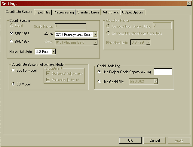
In order process GPS vectors, the coordinate system must be set to
'SPC 1983' with the appropriate state plane zone. The 'Coordinate
System Adjustment Model' must be set to the 3D Model. With the 3D
model,
horizontal units and vertical units must be the same in regards to
output and total station raw data. Geoid modeling may or may not be
important depending on the extent of the project and the accuracies
required. The most accurate results are typically obtained by using a
'Geoid File' set to GEOID03.

Note: The sample tutorial project has the input raw file in the
default
data folder of C:\Carlson2007\Data. If you have a different data
directory, then set the correct data file by highlighting the default
file, pick Delete and then pick Add and select GPSAndTS.cgr (C&G
format raw file) from
your data folder. Do the same for the GPS Vector files of GPSAndTS1.gps
and GPSAndTS2.gps.
None of the settings in this screen are specific to processing GPS
vectors. See the manual for details on the settings in the 'Adjustment'
dialog box.
3 Following is
the
main SurvNET window. To process the data chose the Process/Network
Adjustment option.
The project should process and converge and the following windows
should be displayed.
Let's review sections of the report that are unique to the processing
of GPS vectors and the 3D model.
Notice that now that we are working
with a specific datum instead of an assumed coordinate system that
latitude/longitude, state plane coordinates and geocentric coordinates
are all displayed.
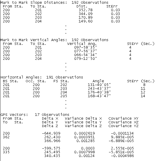
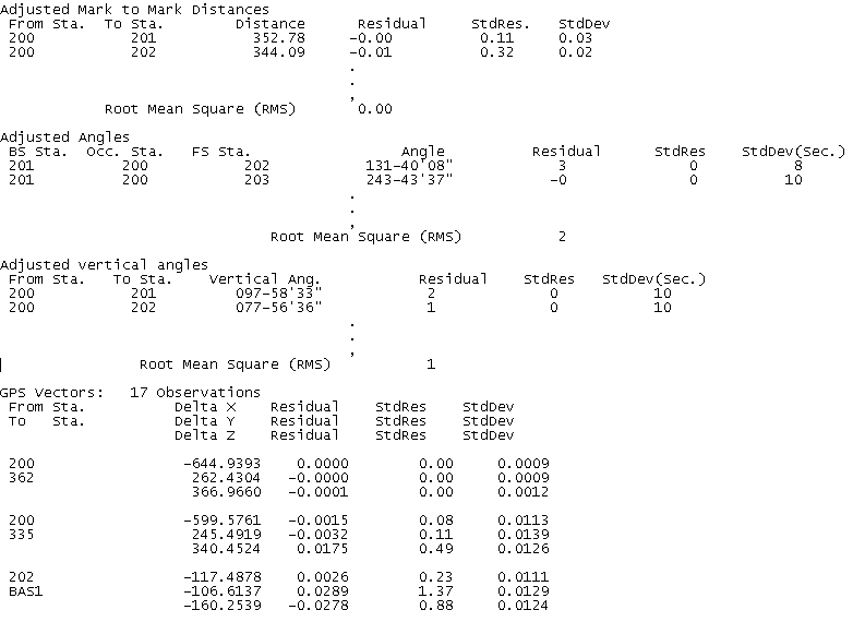
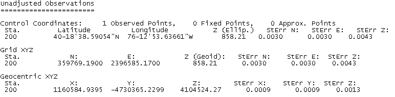
In the above unadjusted
observations section of the report,
notice that
distances have been converted to mark to mark distances. Note that
vertical angles are now treated as measurements in the 3D model. And
lastly, notice that the GPS vectors are also displayed. The GPS vectors
are displayed as delta X,Y,&Z in the geocentric coordinate system.
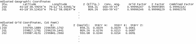
In
the above adjusted coordinate section of the report, notice that
the grid, elevation, and combined factor are displayed with the
adjusted geographic coordinates.